Modelling in Urban and Regional Economics

Alex Anas

• Publisher: Taylor & Francis
• Year: 2013
• ISBN:
  9781136460852
• Edition: 1
• Topic: Business
• Subtopic: Business General
• Index: Business

This title provides a comprehensive, critical coverage of the progress and development of mathematical modelling within urban and regional economics over four decades.

1. MONOCENTRIC MODELS

In this section we will examine the application of simulation to a number of themes in monocentric analysis. Each theme represents an area of policy or scientific interest in which prior analytical exploration quickly reached its limits and thus the application of simulation was warranted. In reviewing these themes, we will indicate why analytical investigation failed in answering the key questions and thus why numerical simulation was necessary. We will focus on what was learned from the simulations and to what extent the new knowledge enriched our understanding of reality and our insight into important policy questions. Monocentric analysis has done well to illustrate the complementarity between theory and simulation: pondering simulation results has yielded insights and generated hypotheses that stimulated theoretical develoments. We will also consider the quality of the artificial or empirical data used in the simulations, although in most cases little confidence can be placed in these data. Finally, we will examine the literature on computational methods for solving general equilibrium monocentric models. This literature emerged in the mid seventies in response to the growing trend toward numerical solutions at that time.

1.1. Income and urban location

An important result in monocentric theory is the location of different income groups within the suburban ring. Beckmann [29] examined this problem under the assumption that all households, regardless of income, had the same Cobb–Douglas utility function defined over a composite commodity purchased at the center and the size of their land plots purchased at their residential location. He also assumed that all households, regardless of income, faced the same transport cost function. The income distribution was a continuous function: the Pareto distribution. The analytically obtained result was simply that at equilibrium a household’s distance from the center increased with the household’s income. In 1974, Wheaton [176] formalized the well understood comparative statics of a monocentric city with a single income group and absentee landlords, and Hartwick, Schweizer and Varaiya [77] generalized Wheaton’s analysis to a monocentric city with a given number of households in each income group. All income groups had different but predetermined incomes and the same utility function (defined over the composite commodity and lot size). A significant but very plausible restriction on the utility function was that land was a normal good. Under these assumptions, the authors showed that the distance of a household’s ring from the center increases as the household’s income increases regardless of the precise income distribution. Furthermore, they performed a full comparative static analysis examining the effect of exogenous changes on the relative welfare and land consumption of the households. An important result in this respect is that increasing the income of the richest class enables it to expand outward by buying more land. This reduces competition for more central land enabling the poorer classes to also expand outward and improve their utility levels. Conversely increasing the income of the poorer classes reduces the welfare of the rich, because it pushes the rich outward raising their transport costs. More recently, Pines and Sadka [136] generalized Wheaton’s [176] comparative statics analysis to a fully closed city, with a single income group, in which aggregate land rent is redistributed equally among the residents. While they reestablish most of Wheaton’s results, they show that the city’s land area may decrease when population increases.

These analytical results ignore the fact that households of different income cannot possibly have identical preferences. As incomes increase preferences also change and it does not follow that the bid rent gradients for land become flatter functions of distance from the center with an increase in income. The question of the relationship between preferences, bid rents and various residential classes arose at the University of Pennyslvania in the late sixties where Britton Harris was attempting empirical applications of the Herbert and Stevens model [83], (see Section 3.3). This led to a Ph.D. dissertation by Wheaton [175] who examined the question empirically and later published some estimates of bid rent functions for the San Francisco area from a home interview sample collected in 1965 [180]. These results are subject to some statistical biases which are discussed in Anas [4; Ch. 1]. Nevertheless they were the first attempt to measure marginal rates of substitution among attributes such as the number of rooms, lot size, housing age and travel time. The empirical results showed some important differences in preferences (coefficients of utility functions) by income. The assumption of preferences invariant across income groups was no longer reasonable to maintain within urban economics, although it remains a mainstream implicit assertion in economic theory.

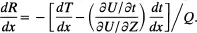
An insight which grew out of Wheaton’s analysis is that the degree of the flattening of a bid rent curve by income depended crucially on two factors: “the preference for land or housing floor space” and “the value of commuting time.” To see this consider that the household maximizes a utility function defined over Z, the composite commodity, Q, lot size, and t, time of travel to the center. Thus, we have the utility function U(Z, Q, t) and the constraints Y – Z – RQ – T(x) = 0 and H – t(x) – L(x) = 0. Here, T(x) and t(x) are the exogeneously given travel cost and travel time functions of distance x, both of which increase with distance. Y is income and H is the total time budget to be divided between travel and leisure, L. Since t(x) is exogeneous and H fixed, L(x) is determined as a residual. R is the bid rent of the household, which is an indifference curve between distance and rent. To see how this varies with distance we impose the conditions dU = 0 and dY = 0 and we obtain from these that

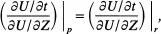
The term in ( . ) is the “value of commuting time,” or marginal rate of substitution between travel time and Z and is negative since ∂U/∂t < 0 by assumption. Since dT/dx and dt/dx are both positive it follows that dR/dx <0. If rich (r)and poor (p) have the same utility function then,

when the utility function is evaluated at the same Z, Q and t for both rich and poor. If

is the border between rich and poor, then it follows from the equation for dR/dx and the assumption that land is a normal good that Q(

)_r > Q(

)_p and thus that the bid rent function for the rich at

is flatter than that for the poor at

. If, however, we wish to take one step closer to realism we ought to recognize that the rich have higher values of time than do the poor, at the same Z, Q and t because they have different utility functions. This tends to make the bid rents of the rich steeper with distance favoring a more central location for them unless their preference for land increases sufficiently faster with income than their dislike for commuting (i.e. their value of time).

Wheaton [179] selected coefficients from his constant elasticity of substitution utility functions which he had estimated with the Bay Area data [180] and performed a simulation with five income groups in a monocentric setting parameterized to have a rough resemblance to the Bay Area. The value of time and the preference for land were the only two factors included in the utility functions, which were different by income group. The way such a simulation works is as follows: bid rent functions are computed for each income group given arbitrary levels of utility. One then orders the groups by the steepness of their bid rent functions in terms of their distance from the center and then computes to see if the ring which they can claim by being the highest bidders is wide enough to accommodate the quantity of land which they demand. One iterates this procedure by adjusting the levels of utility and recomputing the bid rent functions until the quantity of land demanded by each group is equal to the land allocated to that group at equilibrium in the ring reserved for that group. Thus, all households find a location at equilibrium. When one cannot preorder bid rent functions by steepness (because the elasticity of substitution varies between groups) the above procedure can be repeated by trial and error to find the order of each group at equilibrium.

Wheaton’s simulation showed that despite differences in values of time and preferences for land caused by income, the five groups in equilibrium did order themselves according to increasing distance by income. This pattern, however, was not very stable: small perturbations within the estimated standard errors of the utility coefficients caused rich and poor households to flip locations in some cases. Wheaton conjectured that this instability was due to the fact that the preference for public goods, which increases by income, was not in the utility functions. Since the supply and quality of public goods increases with distance due to historical trends, the presence of public goods stabilizes a decentralized location for the rich.

Wheaton’s conjecture remains a plausible but untested proposition. There has been relatively little interest in measuring the preference for public goods and services and no interest in pursuing further the question introduced by Wheaton. It may be observed that in many Latin American and other Third World cities, the rich often occupy central locations while the poor who have low values of time live in the “suburbs” (often squatter settlements) and commute by foot, bicycle or bus, inexpensive but time consuming means of transportation. It is also true, in many of these cities, that central locations have better public services and locational prestige than surrounding areas. It would appear that future work in monocentric simulation would do well to explain the location of different groups by income in an international context to see if different observed location patterns result from different parametrizations of the same theoretical model.

Analytical answers are difficult or nearly impossible to obtain when transport cost and travel time depend on income even if the utility function is constant with income. This issue arose in a paper by Wheaton [178] who conjectured incorrectly that the welfare results established by Hartwick, Schweizer and Varaiya [77] could be generalized to cases where transport cost depended on income. In such cases, Wheaton argued, the rich can have a steeper bid rent gradient, thus locating near the center. Increasing their income would increase their “value of time” making their bids even steeper and reducing competitive land market pressure on the surrounding poor, and thus raising the welfare of the poor. Similarly, increasing the income of the surrounding poor would steepen their bids putting pressure on the centrally located rich, and reducing their welfare. Arnott, MacKinnon and Wheaton [23] later investigated this problem and found two numerical counterexamples by means of monocentric simulation. These are based on the observation that the steepening of the bid rent gradient which occurs because transport costs depend on income, may be more than offset by an upward shift in the bid rent gradient which occurs because land is a normal good. This sort of analysis illustrates the use of simulation to check out a theoretical conjecture based on limited analytical models or faulty intuition. The insight derived from such “checks” is often impressive relative to the low cost of the simulation.

1.2. Congestion and the use of land for roads

The spatial effects of the urban traffic congestion externality forms a celebrated theme within theoretical urban economics. This is probably the most analyzed and overworked problem in both the theoretical and simulation literatures. It is also perhaps the only problem where numerical simulations have proved to be indispensable in firming up the theory. It is a theoretically important problem because it demonstrates the treatment of the theory of the second best in a spatial, urban context.

Traffic congestion arises because households living at different distances away from the center of the city arrive at work and leave for home at roughly the same time. Given a radial road network with certain road width, traffic would pile up into queues. However, in these stylized theoretical models the queueing aspect which stems from a traffic engineering perspective is neglected. Instead, travel cost and/or travel time on a short segment of a road during the rush hours is assumed to be an initially flat but later increasing (and strictly convex) function of the total traffic flowing through that road segment during the rush hour divided by the width (or capacity) of the road segment. This rather crude assumption is the same in the case of realistic network models in transportation planning. In that context, the assumption does much more violence than it does in the case of a monocentric city (see Section 3.1).

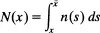
Analytically, the congestion phenomenon in a monocentric city is handled as follows. Let n(x) be the number of households living at the thin annulus of width dx, x miles from the center. Then the number living beyond this radius is given by the integral,

with

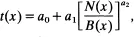
the edge of the city where the urban and agricultural land rents are equal. N(x) is the volume of traffic (or flow) that must pass the circle at radius x, assuming that each household generates one vehicle trip. Then, the private (average) travel time (or travel cost) incurred by each vehicle in crossing the thin annulus of width dx at x is given by a function of the form,

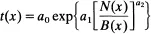
where t(x) is the per mile cost or time, a₀, a₁, a₂ are positive constants and B(x) is the quantity of land in the thin annulus at x reserved for roads or the “road capacity” at x. Cost or time per mile is made a strictly convex increasing function of traffic volume N(x) by choosing a₂ > 1. The above function is almost universally employed and corresponds to the Bureau of Public Roads function employed in practical network equilibrium models. In that function, a₁ = 0.15 and a₂ = 4.0. An exception to the above function is the alternative,

where a₀, a₁ > 0 and a₂ ≥ 1. This was introduced by Arnott and MacKinnon [22]. They employed this function because the elasticity of private congestion with respect to flow exceeds unity and because the ratio of the marginal congestion externality to private congestion is an increasing function of flow. Arnott and MacKinnon refer to these two properties as stylized facts proposed by Solow [156] and Vickrey [171] respectively.

The traffic congestion problem in long run monocentric analysis takes several forms. One is to take as given a reasonable allocation of land to roads described by the function B(x). Given this predetermined B(x) one then solves for the usual land use equilibrium rent and population density gradients and also for the transport expenditure gradient t(x) under the assumption that vehicles incur their private average expenditure at every distance x. This is a second best analysis in two respects: because it takes B(x) as predetermined, and essentially arbitrary, and because it assumes that there is no congestion toll to extract from each vehicle the marginal expenditure it imposes on itself and on other vehicles. It is known from first best analysis that each vehicle should incur not its average cost t(x) but t(x) + N(x)[∂t(x)/∂N(x)], its full marginal expenditure. In a city of households with identical preferences this marginal cost pricing strategy maximizes the common long run equilibrium utility level, given a road width function B(x). The second form of the problem is to determine, within the analysis, the function B(x), i.e. an allocation of land to roads in the first best or second best sense. Again, the first best...

Table of contents

• Cover
• Title
• Copyright
• Contents
• Introduction to the Series
• Introduction
• 1. Monocentric Models
• 2. Non-Economic Beginnings
• 3. Mathematical Programming
• 4. Econometric Models
• 5. Regional and Interregional Models
• Conclusions
• References
• Index