Volatility Surface and Term Structure

High-profit Options Trading Strategies

Kin Keung Lai, Jerome Yen, Shifei Zhou, Hao Wang

• Publisher: Routledge
• Year: 2013
• ISBN:
  9781135006983
• Edition: 1
• Topic: Business
• Subtopic: Business General
• Index: Business

This book provides different financial models based on options to predict underlying asset price and design the risk hedging strategies. Authors of the book have made theoretical innovation to these models to enable the models to be applicable to real market. The book also introduces risk management and hedging strategies based on different criterions. These strategies provide practical guide for real option trading.

This book studies the classical stochastic volatility and deterministic volatility models. For the former, the classical Heston model is integrated with volatility term structure. The correlation of Heston model is considered to be variable. For the latter, the local volatility model is improved from experience of financial practice. The improved local volatility surface is then used for price forecasting. VaR and CVaR are employed as standard criterions for risk management. The options trading strategies are also designed combining different types of options and they have been proven to be profitable in real market.

This book is a combination of theory and practice. Users will find the applications of these financial models in real market to be effective and efficient.

1
Introduction

Stock options trading is a new way of stock trading developed in the 1970s, commonly used in the United States since the early 1990s. A stock option is a right to buy or sell a certain stock at a fixed price within a certain period of time. The buyer is not given the stock itself but the right to buy it at an agreed price.

Execution of an option in options trading is a process where the buyer decides whether to buy or sell the underlying asset at the price the seller and the buyer have agreed. The seller can only passively accept the compliance obligations. Once the buyer asks to execute the option contract, the seller must fulfill their obligations and settle the position specified in the option contract. Hence, the rights and obligations between the seller and the buyer are not equal. The underlying assets of options include commodities, stocks, stock index futures contracts, bonds, and foreign exchange.

The underlying asset of stock index options is the spot index. For example, in the case of the currently popular European option, buyers and sellers directly settle the option contract by cash for stock index options when these options expire. For real option trading, the buyer of a stock index option can only execute the buy right when the option generates the floating profit (earnings greater than the transaction fees) and foregoes the right when there is a loss (including the case where earnings are less than the transaction fee). Hence, there is less risk for the option buyer.

Stock index options sellers face the risk of loss only when they have to passively execute an option contract. However, as long as the premium that sellers collect from buyers can cover the losses, they can hedge the risk of losses. Based on volatility calculated from the stock index and stock index futures contracts, options sellers are able to control the risk of losses to a ninety-five percent confidence level by collecting a conservative premium rate of ten to fifteen percent.

Compared with commodity options, the execution of stock index options and stock index futures are two independent delivery processes. The underlying asset of stock index futures contracts is the spot price index. The stock index is usually composed of a basket of stocks. Commonly, the cash mode is used for settlement of stock index options. That is, the gains and losses of stock index investors are settled by cash at the maturity date of futures contracts.

The execution of stock index options is similar to stock index futures, which can be divided into two modes, US and European. Since the underlying asset of stock index options is also the spot stock index, stock index options are converted into stock index futures on the execution date (US mode) and are exercised with futures, such as the small Chicago Mercantile Exchange (CME) Standard & Poor’s (S&P) 500 index futures and options. The European option is directly executed with cash at maturity, such as the CBOE S&P 500 Index options. However, for European options, the market price usually contains intrinsic value and time value. The intrinsic value is the expected value between the underlying asset price and the strike price at maturity. Hence, in this book, we make use of the market option price and do not discuss the intrinsic and time value of option prices in detail. The option price is also referred to as the market option price by default.

Options trading based on futures can provide a hedging function for the futures trader. To format a multi-level, especially low-risk high-yield portfolio in the futures market, you need to take advantage of options. To reduce the trading risk of futures investors, to expand the scope of market participants, and to improve market stability and liquidity also requires options. In addition, options can provide hedging tools for addressing risk in contractual agriculture and to protect farmers’ revenue. The US government encouraged farmers to successfully combine their government subsidy with the options market so as to transmit the huge risks of the agricultural market to the futures market. This policy not only reduces the government’s fiscal expenditure but also stabilizes agricultural production and effectively protects farmers’ benefits.

In addition to hedging, stock index options also contain certain market information from participants. During the options trading process, buyers and sellers provide bid and ask prices for options. These prices contain views of buyers and sellers about what the underlying asset price is expected to be at the maturity date. Black and Scholes (1973) proposed that implied volatility, calculated from options prices, reflects market information. If the implied volatility of a put option is large, it means market participants are panicky about the future market trend. Conversely, if the implied volatility of a call option is large, this indicates that the market will go up in the near future. Therefore, the study of option implied volatility is significant and beneficial.

1.1 Implied volatility

The implied volatility of an option contract is volatility of price of the underlying asset which is implied in the price of the option. Implied volatility varies with different strikes and time to maturities. For a given time to maturity, the implied volatility varies with strikes; for a given strike, the implied volatility varies with different maturities. To price European options, Black and Scholes (1973) proposed that the price of underlying assets satisfies the following:

where μ is the mean value of historical price, σ is the constant variance of the underlying asset’s price, and W represents a standard Wiener process. From Ito’s Lemma, the logarithmic of the underlying price should follow the formula:

Therefore, the logarithmic of the underlying price follows a normal distribution. However, when applying this theory into practical market options, the normal distribution expresses the phenomenon of a fat tail at both sides of the distribution. Black and Scholes proposed this model based on the following assumptions: (1) no dividend before the option maturity; (2) no arbitrage; (3) a constant risk-free interest rate; (4) no transaction cost or taxes; (5) divisible securities; (6) continuous trading; and (7) constant volatility. For a given time during the trading day, if the market releases the option price, the option volatility can be calculated by inverting the Black–Scholes formula.

On the one hand, if the time to maturity is fixed, volatility smile is defined as a curve that the implied volatility changes with different strikes. In a long-observed pattern, the volatility smile looks like a smile. The implied volatility of an at-the-money option is smaller than that of in- or out-of-the-money options. When the implied volatility of an out-of-the-money put option is larger than that of an out-of-the-money call option, this curve is called implied volatility skew. Zhang and Xiang (2008) defined the concept of “moneyness” as the logarithm of the strike price over the forward price, normalized by standard deviation of expected asset return as follows:

where σ is the historical volatility of the underlying asset price; τ is the time to maturity; K is strike price; F is the forward index level. Then, implied volatility smirk is defined as employing the moneyness as an independent variable. Implied volatility changes according to moneyness.

On the other hand, if implied volatilities with different strikes and a given maturity are combined together under a certain weighted scheme, then the implied volatility term structure can be defined as a curve that implied volatilities change with different maturities. When the implied volatilities of call options and put options are calculated, we obtain a call implied volatility curve and a put implied volatility curve. The spread between call and put curve is called call–put term structure spread. This spread contains certain market information.

When implied volatility of put term structure is larger than that of call term structure, market participants worry about the market on the maturity date. If these two curves cross, there are two conditions. First, when implied volatility of the put curve is larger than call curve before the cross point and smaller after the cross point, it means the market trend may reverse in a short term and go up. Second, when implied volatility of call curve is larger than the put curve before the cross point and smaller after the cross point, it means the market trend may reverse in a short term and go down. Finally, when the implied volatility of call term structure is larger than that of put term structure, the view from investors is that the market still goes up. By using this functionality of term structure, we can employ the term structure to predict the underlying asset price efficiently, which is discussed in greater detail in Chapters 2 and 9.

1.2 Local volatility model

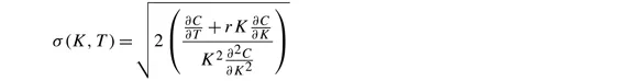
Local volatility also performs well in forecasting the underlying asset price. Local volatility is an instantaneous volatility that is a function of time t and underlying asset price S_t. Typically, Dupire (1994) presented a deterministic equation to calculate the local volatility from option price based on the assumption that all call options with different strikes and maturities should be priced in a consistent manner.

Nevertheless, this deterministic function suffers two weaknesses. First, because local volatility is a function of both strike and time to maturity and it is possible that not all strikes are available at each time to maturity, the number of local volatilities is finite and is usually not enough for further calculation and applications. As a result, researchers are inclined to use interpolation to obtain a series data of local volatility for further calculations. In this way, the algorithm of interpolation becomes very important because a weak algorithm results in problem of inadequate precision. Second, there is the intrinsic problem of the Dupire’s equation. The indeterminancy of the equation may cause local volatility to be extremely large or very small. In Chapter 6, we propose a mean-reversion process to overcome these faults and improve the model. As local volatility is a function of time and underlying asset price, it has the ability of predicting the underlying asset price if we can construct the local volatility surface.

1.3 Stochastic volatility model

In the stochastic volatility model, volatility is considered as a stochastic process. The stochastic volatility model assumes that the underlying asset price follows a geometric Brownian process. In the Black–Scholes model, volatility is assumed to be constant over the time to maturity. However, this can explain the phenomenon that volatility smile and skew vary with different strikes. The stochastic volatility model can solve this problem. Typically, Heston (1993) proposed a model which considers the underlying asset price process and the volatility process as random processes. Moreover, these two processes have a constant correlation.

The underlying level process of Heston model is composed of two terms, the price drift term and the volatility with random motion term. The volatility process is also composed of two terms, a volatility drift with mean reversion functionality and a volatility of volatility with random motion. The model is formulated as follows:

where θ is the long-run mean level of volatility, κ is the speed of instant volatility returning to long-run mean level, and σ is volatility of volatility. These three parameters satisfy the condition of 2κ_tθ > σ² and ensure the process of V_t is strictly positive. Furthermore, W₁ and W₂ are two standard Wiener processes and have a correlation of ρ.

The Heston model has been widely applied in equities, gold, and foreign exchange markets. Furthermore, many extended models based on the Heston model have been propose...

Table of contents

• Cover
• Title
• Copyright
• Contents
• List of figures
• List of tables
• Preface
• 1 Introduction
• 2 A novel model-free term structure for stock prediction
• 3 An adaptive correlation Heston model for stock prediction
• 4 The algorithm to control risk using options
• 5 Option strategies: evaluation criteria and optimization
• 6 A novel mean reversion-based local volatility model
• 7 Regression-based correlation modeling for the Heston model
• 8 Index option strategies: comparison and self-risk management
• 9 Call–put term structure spread-based Hang Seng Index analysis
• Notes
• References
• Index