Ordinary and Partial Differential Equation Routines in C, C++, Fortran, Java, Maple, and MATLAB

H.J. Lee, W.E. Schiesser

• Publisher: Chapman and Hall/CRC
• Year: 2003
• ISBN:
  9781135437794
• Edition: 1
• Topic: Mathématiques
• Subtopic: Mathématiques générales

This book provides a set of ODE/PDE integration routines in the six most widely used computer languages, enabling scientists and engineers to apply ODE/PDE analysis toward solving complex problems. This text concisely reviews integration algorithms, then analyzes the widely used Runge-Kutta method. It first presents a complete code before discussin

1

Some Basics of ODE Integration

The central topic of this book is the programming and use of a set of library routines for the numerical solution (integration) of systems of initial value ordinary differential equations (ODEs). We start by reviewing some of the basic concepts of ODEs, including methods of integration, that are the mathematical foundation for an understanding of the ODE integration routines.

1.1 General Initial Value ODE Problem

The general problem for a single initial-value ODE is simply stated as

(1.1)(1.2)

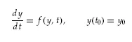
where

y = dependent variable

t = independent variable

f (y, t) = derivative function

t0 = initial value of the independent variable

y0 = initial value of the dependent variable

Equations 1.1 and 1.2 will be termed a 1x1 problem (one equation in one unknown). The solution of this 1x1 problem is the dependent variable as a function of the independent variable, y(t) (this function when substituted into Equations 1.1 and 1.2 satisfies these equations). This solution may be a mathematical function, termed an analytical solution.

To illustrate these ideas, we consider the 1x1 problem, from Braun¹ (which will be discussed subsequently in more detail)

(1.3)(1.4)

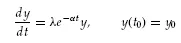
where λ and α are positive constants.

Equation 1.3 is termed a first-order, linear, ordinary differential equation with variable coefficients. These terms are explained below.

See Table

The analytical solution to Equations 1.3 and 1.4 is from Braun:¹

(1.5)

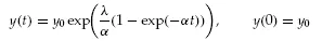
where exp(x) = e^x. Equation 1.5 is easily verified as the solution to Equations 1.3 and 1.4 by substitution in these equations:

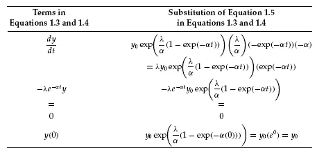
thus confirming Equation 1.5 satisfies Equations 1.3 and 1.4.

As an example of a nxn problem (n ODEs in n unknowns), we will also subsequently consider in detail the 2x2 system

(1.6)

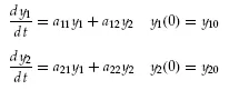
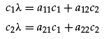
The solution to Equations 1.6 is again the dependent variables, y_1, y₂, as a function of the independent variable, t. Since Equations 1.6 are linear, constant coefficient ODEs, their solution is easily derived, e.g., by assuming exponential functions in t or by the Laplace transform. If we assume exponential functions

(1.7)

where c₁, c₂, and λ are constants to be determined, substitution of Equations 1.7 in Equations 1.6 gives

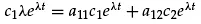
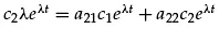
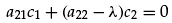
Cancellation of e^λt gives a system of algebraic equations (this is the reason assuming exponential solutions works in the case of linear, constant coefficient ODEs)

or

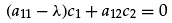
(1.8)

Equations 1.8 are the 2x2 case of the linear algebraic eigenvalue problem

(1.9)

(A − λI)c = 0

where

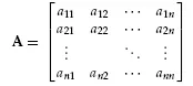
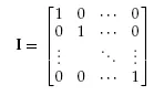
n = 2 for Equations 1.8, and we use a bold faced symbol for a matrix or a vector.

The preceding matrices and vectors are

A nxn coefficient matrix

I nxn identity matrix

c nx1 solution vector

0 nx1 zero vector

The reader should confirm that the matrices and vectors in Equation 1.9 have the correct dimensions for all of the indicated operations (e.g., matrix additions, matrix-vector multiples).

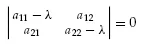
Note that Equation 1.9 is a linear, homogeneous algebraic system (homogeneous means that the right-hand side (RHS) is the zero vector). Thus, Equation 1.9, or its 2x2 counterpart, Equations 1.8, will have nontrivial solutions (c ≠ 0) if and only if (iff) the determinant of the coefficient matrix is zero, i.e.,

(1.10)

|A − λI| = 0

Equation 1.10 is the characteristic equation for Equation 1.9 (note that it is a scalar equation). The values of λthat satisfy Equation 1.10 are the eigenvalues of Equation 1.9. For the 2x2 problem of Equations 1.8, Equation 1.10 is

or

(1.11)

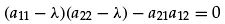
Equation 1.11 is the characteristic equation or characteristic polynomial for Equations 1.8; note that since Equations 1.8 are a 2x2 linear homogeneous algebraic system, the characteristic equation (Equation 1.11) is a second-order polynomial. Similarly, since Equation 1.9 is a nxn linear homogeneous algebraic system, its characteristic equation is a nth-order polynomial.

Equation 1.11 can be factored by the quadratic formula

(1.12)

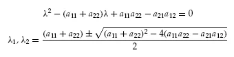
Thus, as expected, the 2x2 system of Equations 1.8 has two eigenvalues. In general, the nxn algebraic system, Equation 1.9, will have n eigenvalues, λ₁, λ₂, . . ., λ_n (which may be real or complex conjugates, distinct or repeated).

Since Equations 1.6 are linear constant coefficient ODEs, their general solution will be a linear combination of exponential functions, one for each eigenvalue

(1.13)

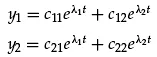
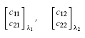
Equations 1.13 have four constants which occur in pairs, one pair for each eigenvalue. Thus, the pair [c₁₁ c₂₁]^T is the eigenvector for eigenvalue λ₁ while [c₁₂ c₂₂]^T is the eigenvector for eigenvalue λ2. In general, the nxn system of Equation 1.9 will have a nx1 eigenvector for each of its n eigenvalues. Note that the naming convention for any constant in an eigenvector, c_{i j}, is the ith constant for the jth eigenvalue. We can restate the two eigenvectors for Equation 1.13 (or Equations 1.8) as

(1.14)

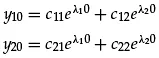
Finally, the four constants in eigenvectors (Equations 1.14) are related through the initial conditions of Equations 1.6 and either of Equations 1.8

(1.15)

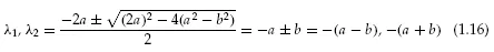
To simplify the analysis somewhat, we consider the special case a₁₁ = a₂₂ = −a, a₂₁ = a₁₂ = b, where a and b are constants. Then from Equation 1.12,

(1.16)

From the first of Equations 1.8 for λ = λ₁

(a₁₁ − λ₁)c₁₁ + a₁₂c₂₁ = 0

or

(−a + (a − b))c₁₁ + bc₂₁ = 0
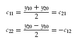
c₁₁ = c₂₁

Similarly, for λ = λ₂

(a₁₁ − λ₂)c₁₂ + a₁₂c₂₂ = 0

or

(−a + (a + b))c₁₂ + bc₂₂ = 0
c₁₂ = −c₂₂

Substitution of these results in Equations 1.15 gives

y₁₀ = c₁₁ − c₂₂
y₂₀ = c₁₁ + c₂₂

or

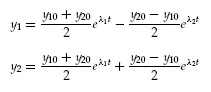
Finally, the solution from Equations 1.13 is

(1.17)

Equations 1.17 can easily be checked by substitution in Equations 1.6 (with a₁₁ = a₂₂ = −a, a₂₁ = a₁₂ = b) and application of the initial conditions at t = 0:

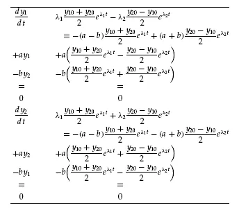
For the initial conditions of Equations 1.6

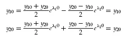
as required.

The ODE problems of Eq...

Table of contents

• Cover Page
• Title Page
• Copyright Page
• Preface
• 1
• 2
• 3
• 4
• 5
• Appendix A
• Appendix B
• Appendix C
• Appendix D
• Appendix E
• Appendix F