Debugging Embedded Microprocessor Systems

Stuart Ball

• Publisher: Newnes
• Year: 1998
• ISBN:
  9780080503806
• Topic: Technology & Engineering
• Subtopic: Microelectronics
• Index: Technology & Engineering

Debugging Embedded Microprocessor Systems provides techniques for engineers, technicians, and students who need to correct design faults in embedded systems. Using real-world scenarios, designers can learn practical, time-saving ways to avoid and repair potentially costly problems. Prevention is stressed.

In this book, the author addresses hardware and software issues, including up-front design techniques to prevent bugs and contain design creep. Practical advice includes descriptions of common tools which can be used to help identify and repair bugs, as well as test routines. RTOS and embedded PC environments are also covered.

Each chapter of Debugging Embedded Microprocessor Systems opens with an example design problem which illustrates real-world issues such as design changes, time pressures, equipment or component availability, etc. Case studies of past debugging projects are presented in the final chapter.

• Addresses real-world issues like design changes, time pressures, equipment or component availability
• Practical, time-saving methods for preventing and correcting design problems
• Covers debugging tools and programmer test routines

1

Tools for Debugging Embedded Systems

Cody Horton stuck his head into the office. Matt Grover was on the telephone, but waved Cody to the empty chair beside his desk.

“Tell them to look at the parameters in the configuration table,” Matt said to whomever was on the other end of the conversation. “I bet you’ll find that one of them has been corrupted.”

Cody looked around the office. A pen-and-ink caricature of Matt and someone, presumably his wife, was thumbtacked to the wall beside the desk. A stack of CDs sat in a plastic case beside the computer. He scanned the titles of the books in the bookcase, noting the usual assortment of IC databooks and application manuals. A red book with yellow lettering caught his eye, and he pulled it from the bookcase. Morals of a Politician, Compassion of a Rattlesnake was the title, followed by the subtitle: Ethics in Today’s Business Environment.

Cody idly thumbed through the book before replacing it in the bookcase. He scanned the room again. A small circuit board was mounted on a wooden stand on one corner of Matt’s desk. The board was fully populated with components except for an empty PLCC socket in the middle.

Matt hung up the telephone and Cody leaned across the desk and held out his hand.

“Cody Horton,” he said. “I just started here a couple of months ago.”

“I’ve seen you around,” Matt replied. “What can I do for you?”

Cody pointed to the PC board on the stand. “What’s that?” he asked.

Matt smiled. “I’ll tell you the story about that sometime,” he replied.

Cody shrugged and unrolled a schematic onto Matt’s desk. “Are you familiar with the project we’re doing for Quad Systems?” he asked.

Matt nodded. “I did some of the early estimates. Fifty test stations.”

“One of the later additions to the contract specified that we provide hardware for in-circuit programming of the EPROMs on the boards. All the parts are soldered in the production versions so the machine vibration won’t shake them out. Anyway, I got the task of designing the programmer. It’s the first embedded design I’ve tackled on my own. Someone suggested that I let you look the design over before I start working on the prototype.”

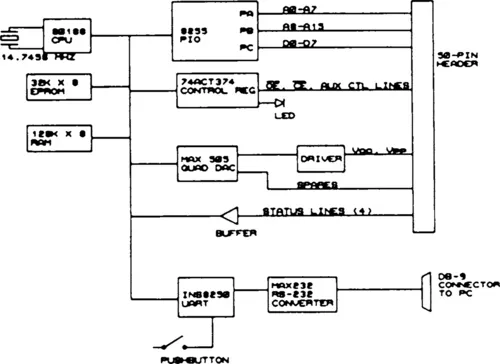
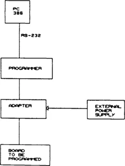
“Do you have a block diagram?” Matt asked.

In response, Cody pulled the last page from the stack of schematics and placed it on top. Matt studied the diagram for a few moments. “How do the boards plug into the programmer?” he asked.

“There’s an adapter board for each board to be programmed. The adapter plugs into the 50-pin connector on the programmer and then into whatever connector is on the target board. Some of the boards were short of real estate, so we have to load addresses and data serially or something like that. We may use a short ribbon cable in some cases.”

Matt took a marker out of his desk drawer and handed it to Cody. “Draw me a picture of the system,” he said.

Figure 1.1 Programmer Block Diagram

Cody nodded and quickly sketched out a block diagram.

“What kind of PC?” Matt asked.

“The customer supplies the computer, so I’m trying to make it run on about anything. That’s why I’m limiting the baud rate to 9600. That should let us use anything from a 286 to a Pentium.”

Matt flipped through the schematic pages to the block diagram of the programmer, then took a calculator out of his desk drawer and punched some buttons. “I assume you picked the 14.75 crystal because it divides down to a standard baud rate. Did you make sure that the 16550 can handle the 7.37 MHz from the processor?”

“The UART input clock can go to 8 MHz.”

“What kind of data gets passed over the serial interface?”

“The host computer sends commands and hex data to the programmer, and the programmer sends messages back to the host. The command interface hasn’t been defined. I had planned to let whoever does the PC software supply a user-friendly interface, so the interface in the programmer could be kept fairly simple.”

“Who is writing the firmware?”

“There was supposed to be someone from the software group assigned for the firmware and the PC software, but Josh Underwood said they were pulled off to solve some crisis on another project. I’ll have to do the firmware, but someone else will do the PC software.”

Figure 1.2 System Block Diagram

“Have you added anything for debugging?”

“Like what?”

“Test points, diagnostic outputs, anything like that.”

“I hadn’t really thought about debugging the board.”

Matt nodded again. “So you haven’t thought about what tools you’ll need to debug the design then.”

“No.”

“Do you know what tools we have in the lab?”

“I’ve used a ’scope. Other than that, I don’t know what we have.”

“Do you have a budget to buy any tools with?”

Cody looked sheepish. “No. This entire project was tacked on as kind of an afterthought, so there isn’t much of a budget. I’ve been concentrating on the design itself.”

Matt stood up. “Let’s take a stroll out to the lab and see what’s there.”

Test Equipment

While Matt and Cody take an inventory of test equipment in their lab, we’ll look at the types of test equipment that are used in debugging embedded systems.

Oscilloscope: Most engineers are familiar with the ’scope. It displays a horizontal trace of one or more waveforms, usually in real time.

DSO: A Digital Storage Oscilloscope (DSO, or sometimes Digitizing Oscilloscope) captures the data and stores it in an internal memory. This allows the data to be captured and examined later. A DSO allows infrequent events, such as a pulse that occurs only once every few minutes, to be displayed. An analog ’scope is better at displaying repetitive events than at displaying single events—a single sample of a waveform sweeps across the screen and is gone. A storage ’scope is a special kind of analog ’scope and uses a screen with a long persistence to “freeze” events, but these scopes have been almost universally replaced by the DSO.

A DSO passes the input waveform through an ADC (analog-to-digital converter), which digitizes the signal and then stores the resulting value in memory. Samples are taken at regular intervals, and the signal is reconstructed from the stored data. This method of capturing the waveform gives the DSO some unique limitations.

The first drawback to the DSO is limited memory. If a DSO can hold 1024 samples, then it can store and display 1.024 seconds’ worth of data when sampling at 1 kHz, or 1.024 milliseconds’ worth of data when sampling at 1 MHz. Obviously, the larger the memory, the more you can see at a given resolution.

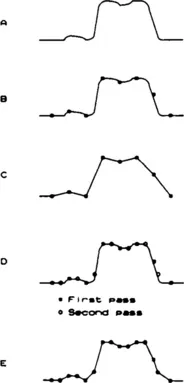
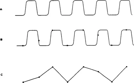
DSOs also have a limitation in reconstructing the waveform. Figure 1.3A shows a waveform as it might be seen on an analog ’scope. Figure 1.3B shows the same waveform with dots where a DSO might capture the data. Figure 1.3C shows how this would be displayed on the DSO screen if the DSO connects the sample points with straight lines. Obviously, there is some distortion in the waveform. A higher sampling rate would improve the reconstructed image, but would also reduce the total sample time that can be stored. It is important to note that the voltages at the indicated sampling points in Figure 1.3B are all that the DSO stores—the waveform between these sample points is filled in by the DSO on the display only.

Figure 1.3 DSO Sampling

Some DSOs can use equivalent time sampling on repetitive waveforms. With this method, each trigger of the DSO causes samples to be taken at the same regular intervals, but each sampling pass starts at a slightly different time with respect to the trigger. Figure 1.3D shows a waveform sampled twice, with the two sample intervals offset by half the sampling time. Figure 1.3E shows the resulting display, which is very close to the original signal in Figure 1.3A. Obviously, the more samples that are taken, the more accurate the reconstructed image will be. A nonrepetitive waveform or a single event cannot be sampled this way, as the DSO gets only one pass at storing the data.

Some DSOs improve the image by reconstructing the display with some type of curve match, such as a sine. This improves the appearance of the display, but it can make the waveforms appear to be better than they really are. Most DSOs that provide this feature also allow straight-line matching.

Aliasing, as shown in Figure 1.4, occurs when the DSO sample rate is too slow to represent the input waveform. When the sweep speed of an analog ’scope is set too slow, the screen will be filled with a signal that contains frequencies obviously too high to examine in detail. A DSO, however, does not capture or display anything that occurs between its regular samples. Figure 1.4A shows a repetitive waveform, such as the clock from a microprocessor. Figure 1.4B shows where a hypothetical DSO might sample the waveform, and Figure 1.4C shows the resulting display. Aliasing can be a real problem, especially if the sample time is very close to a submultiple of the input frequency. When that happens, it may appear that the waveform is correct, but at a frequency that is completely wrong. Anyone who has used a DSO for very long has been bitten by aliasing at least once.

Figure 1.4 DSO Aliasing

Repetition Rate: Because of the time required to display the signal, a DSO typically cannot retrigger as quickly as a good analog ’scope. However, faster processors and memory are closing this gap.

Advantages of DSOs: With all its drawbacks, the DSO is still the instrument of choice...

Table of contents

• Cover image
• Title page
• Table of Contents
• Copyright
• Introduction
• Chapter 1: Tools for Debugging Embedded Systems
• Chapter 2: Adding Diagnostic Helps to the Target System
• Chapter 3: General Debugging Tips
• Chapter 4: Hardware Debug
• Chapter 5: Debugging the Software
• Chapter 6: Debugging the Interrupts
• Chapter 7: Debugging in an RTOS Environment
• Chapter 8: Debugging in an Embedded PC Environment
• Chapter 9: Debugging Scenarios from the Trenches
• Appendix 1: Programmer Test Routines
• Glossary
• Index