An Introduction To Experimental Design And Statistics For Biology

David Heath

• Publisher: CRC Press
• Year: 1995
• ISBN:
  9781135370107
• Edition: 1
• Topic: Mathematics
• Subtopic: Probability & Statistics
• Index: Mathematics

This illustrated textbook for biologists provides a refreshingly clear and authoritative introduction to the key ideas of sampling, experimental design, and statistical analysis. The author presents statistical concepts through common sense, non-mathematical explanations and diagrams. These are followed by the relevant formulae and illustrated by w

1

Why Biologists Need Sampling, Experimental Design and Statistics

Our knowledge of the living world depends upon careful observation and experimentation, followed by analysis and interpretation of the results. Three indispensable tools used in this process are sampling, experimental design and statistical analysis. This chapter examines why they are so important and looks at some of the basic principles.

What Biologists Do

Biology is the study of the living world, a subject which ranges from the molecules that make up cells to the structure and function of whole ecosystems. When the subject was young a biologist such as Darwin could successfully investigate topics as diverse as earthworms, barnacles, orchids and evolution, but as our knowledge has expanded it has become impossible for any individual biologist to deal with the whole of the subject.

Biology has become subdivided into a variety of separate specialised areas or disciplines, with individual biologists restricting themselves to the study of some small part of the subject. There are a number of different ways in which we can describe this subdivision. One is to use the different levels of organization of biological systems, starting at the level of molecules and progressing through cells, organisms and populations, to ecosystems. Such a subdivision is reflected in a range of different sorts of biologists, for example molecular biologists and population biologists. Another way of subdividing the subject is based on whether the organism being investigated is an animal, a plant or a micro-organism. There are biologists who would describe themselves as animal population biologists or plant molecular biologists, with even finer subdivisions and labels based on whether, for example, the animals of interest are vertebrate or invertebrate, insect or mollusc. Alternatively, we could use a scheme based on biological processes such as genetics, development or physiology. This too would produce a corresponding subdivision of biologists into types.

This is not to suggest that biology falls neatly into a number of labelled boxes. It does not! Rather, the divisions are artificial and the borderlines between the disciplines are fuzzy. What it does emphasize is the great diversity of the subject, something which might suggest that the different sorts of biologist have little in common. However, we find that this is not so if we look at the subject from a different angle. In fact all biologists are basically doing the same two things namely answering “What?” and “How?” questions.

“What?” questions involve the description of the characteristics of the particular part of the living world that is of interest, broadly “What is to be found?”. So an animal ecologist might describe the number of individuals in a habitat and a cell biologist might describe the concentration of a specific protein in cells of a certain type at two different stages of the cell cycle. “How?” questions involve an explanation of what has been described, broadly “How can it be accounted for?”. Our ecologist may want to know how a habitat supports the numbers observed. The cell biologist might want to know how the difference in time brings about the difference in protein concentration. As we shall see later on, these two types of question are quite closely related because explanation involves description under specified conditions.

In seeking answers to these two types of question all biologists encounter a similar set of problems, some of which are common to the other sciences, while others are unique to biological systems. It is these problems and the solutions to them which form the subject matter of this book and we start with the basic cause of the trouble – variability.

Variability

Different types of biologists are interested in different sorts of things but they are all involved in making observations on the things of interest and describing them with respect to certain characteristics. Whether we are counting the number of bird species in different woods of a given size, counting the number of individual snails in quadrats on the seashore, measuring the dry weight of individual plants, measuring the concentration of a protein in 10 ml batches of solution or describing the ratio of red to white flowered plants in a genetic cross the observations will have one feature in common – variability.

What this means is that the things of interest, e.g. woods, quadrats, plants, and batches of solution, will not necessarily be identical with respect to the characteristic which is being described. For example not all woods of the same size will have the same number of species, not all individuals of a given plant species will have the same dry weight when grown under the same conditions and not all measurements of protein concentration in 10 ml batches of solution taken from a flask will give the same result. In fact, this feature of biological material is so universal that it gives rise to the general term which is used to refer to characteristics being described. They are called variables. The number of bird species in woods of a given size, the number of individual snails in a quadrat, the dry weight of individual plants, the protein concentration in a 10ml batch of solution and the ratio of red to white flowered plants are all variables.

The basic problem with variability is that it gets in our way when we attempt to describe and explain. We’ll see later why it gets in the way but to understand the problem we first of all need to know why things are variable.

Machines and Techniques – Experimental Variation

The first source of variability is common to all the sciences and is usually referred to as experimental variation. It is variability that is introduced by the experimenter or by the techniques and the equipment used. It arises because of experimental error. Whenever we count or measure anything we are unlikely to do it without error, in other words we will not always count or measure the true value. This may be because our measuring device, be it ruler, pipette or spectrophotometer has inherent limits as to its accuracy. In addition we may use the device in a slightly different way on different occasions, that is our technique may vary.

The simplest way to see how this can happen is to imagine making repeated measurements of exactly the same thing. Take a simple biochemical example which involves measuring the concentration of a chemical in solution (Fig. 1.1). To do this we have to pipette 10 ml of the solution from a flask, add a known quantity of a reagent to produce a coloured end-product at a concentration which is proportional to the concentration of the chemical of interest. The concentration of the colour and hence the concentration of the chemical is measured using a spectrophotometer. If you were to repeat this procedure several times using the same solution, would you get the same answer each time? The chances are that you would not, simply because of variation in the way in which you carry out the procedure on different occasions. Sometimes you will pipette slightly less than 10ml, other times slightly more (Fig. 1.1a) and the quantity of the reagent added will not be exactly the same on different occasions for the same reason (Fig. 1.1b). You may leave the colour to develop for slightly different lengths of time (Fig. 1.1c), there may be slight differences in the optical properties of the different cuvettes (Fig. 1.1d), or the characteristics of the spectro-photometer may change as components age or the mains voltage fluctuates (Fig. 1.1e).

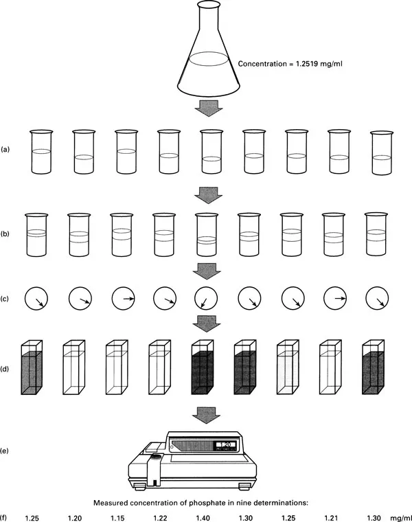
Figure 1.1 Experimental Variation in the Measurement of Phosphate Concentration.

Each potential source of error may, on its own, produce a measurement which is either above or below the true value and, in any one determination of the concentration, errors at different stages of the procedure will be cumulative. Sometimes, by chance, the effects of errors in one direction will be more or less cancelled out by those of errors in the opposite direction, leading to a result fairly close to the true value. On other occasions, again by chance, the majority of errors will all be in one direction, leading to a result which is very different from the true value.

To show you the extent of this type of variability I have included at the bottom of the figure a set of results produced by one person (a first year student). They are concentrations of phosphate in solution measured by just the sort of procedure we have been discussing. The nine determinations were made on the same solution and the variability is obvious! Additional variability would have arisen if nine different students had taken part or if more than one spectrophotometer had been used.

The errors that lead to this variability are not like mistakes in spelling or calculations which, with care, are completely avoidable. Experimental variation is always with us. While it can be reduced by careful experimental technique it can never be completely eliminated. As a result the answer that we obtain will depend on which particular combination of errors our determination is subject to. Our description will be inaccurate.

Variability in Phenotypes and Genotypes

A second source of variability arises from the differences in biochemistry, physiology, morphology and behaviour that exist between individual organisms of the same species. This is something that is very obvious in our own species and it is not hard to find examples in other organisms (Plate 1). Sometimes this type of variability is not apparent on a cursory inspection, however a close study of the individuals concerned will almost always reveal differences between them.

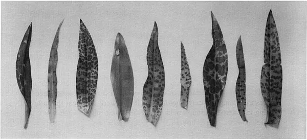
Plate 1 Phenotypic Variability in the Leaves of the Southern Marsh Orchid Dactylorhiza praetermissa.

The almost universal presence of this type of variability is not surprising, considering what we know about the way in which these characteristics are produced. The characteristics of the individual comprise its phenotype, which is the result of the interaction between the individual’s genotype and the environment in which it develops and lives. In sexually reproducing organisms the processes of meiosis and fertilization lead to the continual production of new combinations of genotypes, such that no two individuals are likely to be genetically identical. (There are some obvious exceptions to this such as identical twins, where two individuals have arisen from the same fertilized egg, and plants produced by means of vegetative reproduction. We will meet these and some other exceptions later on because they turn out to be quite useful when we are answering “How?” questions.) The presence of these genetic differences between individuals will lead to phenotypic differences between them, even if they lived in identical environments. This in itself is very unlikely because environments vary in both space and time. Because no two individuals are likely to experience the same set of environmental conditions any differences in the environment experienced by individuals will further increase their phenotypic differences.

The extent to which this will happen depends on the particular characteristic. Some phenotypic differences, such as blood group in our own species, appear not to be affected by the environment. If you have the genes for blood group O, then your phenotype is O irrespective of your environment. Other phenotypic differences between individuals in characteristics such as height, weight, behaviour and susceptibility to disease depend both on the genotype and the environment. As a result the same genotype can produce different phenotypes depending on the environment and, conversely, different genotypes can produce the same phenotype. An individual with genes for large body size will be large if there is plenty of food available, but will be smaller if food is limited; under these conditions it may be the same size as an individual with genes for small size which has access to plenty of food.

These interactions between the genotype and the environment are not restricted to the period of embryonic development, nor do they stop once the individual is an adult. Physiological characteristics such as hormone levels, reproductive state and nutritional state are aspects of an individual’s phenotype which may change from hour to hour, day to day and month to month, because of changes in the environment. For example, human body temperature is said to be 36.8°C, but it differs slightly between males and females and between individuals of the same sex. Also, for a given individual, it varies according to where (in or on the body) it is measured, the time of day and, for females, the stage in the menstrual cycle. It also varies in relation to factors such as the level of physical exertion.

If individuals do differ from one another then, when you describe the characteristic, the answer which you get will depend on which individuals you have looked at. Again we have a problem in describing the variable.

Variability in Space and Time

Characteristics such as the numbers of individuals per unit area of habitat and the number of visits per unit time by pollinators to a flower are also variables. Plate 2 shows a typical pattern of spatial variation in numbers per unit area. In order to understand how this third type of variability arises we need to think about how the organisms came to be where they were.

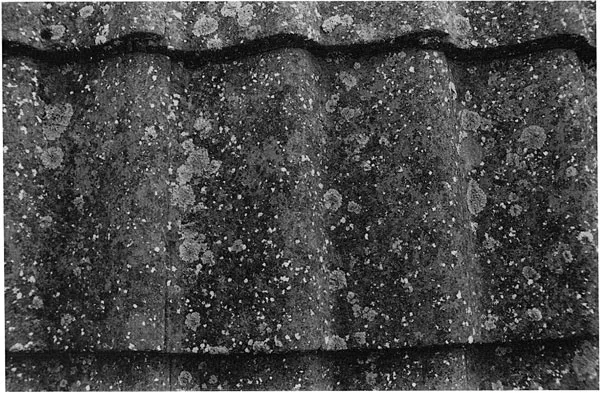
Plate 2 Spatial Variation in Numbers of Lichen Colonies on Roof-Tiles.

Organisms, their seeds, spores and larvae are often passively dispersed by air and water currents and we could imagine them simply “falling out” of the air or water onto the substrate. Contrary to what you might think, this will not lead to the individuals being regularly arranged on the surface because, by chance, some areas will receive more individuals than others. We will look into this in more detail in Chapter 5, but you can demonstrate this effect by simply dropping a handful of something like gravel onto the ground.

For real organisms these chance irregularities will be modified by a variety of factors. For example, eddy currents in the air or water may lead to much higher numbers being deposited in certain areas – think of the way in which the wind can produce piles of leaves. Seeds may tend to fall near the plant that produced them, leading to high numbers of plants clustered around the parent and the same may be true of the offspring of some animals. Finally, animals in their dispersive stage are often capable of exercising choice in where they settle. If the surface is a mosaic of suitable and unsuitable patches then organisms will congregate in the suitable patches, again leading to variation in numbers in different areas. Even if none of this happened and organisms were regularly dispersed at the settlement stage, this is unlikely to persist for long, simply because of the patchy environment. Individuals will survive (and reproduce) better in the suitable patches again producing variation in the numbers from one place to another. Note that one thing which may determine the suitability of a patch is the number of individuals of your own species that are already there.

Rather similar arguments apply to the distribution of events in time. The number of mutations occurring in a population of fixed size will vary by chance from one generation to the next even though the underlying mutation rate is constant. Similarly, if we record the number of pollinator visits to each of 10 identical flowers in a 5-min period, again purely by chance, the number of visits to each flower will not necessarily be the same.

Why Description Needs Statistics

As mentioned earlier, the presence of this variability makes it impossible to describe “things” exactly, that is to put a reliable numerical value to the characteristic of interest. Why is this?

Estimating

First let’s look again at the example of the measurement of phosphate concentration that we were using earlier to illustrate experimental variation....

Table of contents

• Cover
• Half Title
• Title Page
• Copyright
• Contents
• Acknowledgements
• List of tables
• Introduction
• 1. Why biologists need sampling, experimental design and statistics
• 2. Some basic ideas in experimental design and statistical analysis
• 3. Variables, populations and samples
• 4. Describing samples
• 5. Three important models for the frequency distribution of variables
• 6. Tests on a single sample: do the data fit the model?
• 7. Single samples: the reliability of estimates
• 8. Tests on a single sample: association and correlation between two variables
• 9. Tests using two independent samples: are the two populations different?
• 10. Tests for two related samples
• 11. Tests using three or more samples: do three or more populations differ?
• 12. Checklists for the design of sampling programmes and experiments and a key to statistical tests
• Appendix
• Further reading
• Glossary
• Glossary of symbols
• Index