Diffusion MRI

From quantitative measurement to in-vivo neuroanatomy

Heidi Johansen-Berg, Timothy E.J. Behrens

• Publisher: Academic Press
• Year: 2009
• ISBN:
  9780080878515
• Topic: Psychology
• Subtopic: Neuropsychology
• Index: Psychology

Diffusion MRI is a magnetic resonance imaging (MRI) method that produces in vivo images of biological tissues weighted with the local microstructural characteristics of water diffusion, providing an effective means of visualizing functional connectivities in the nervous system. This book is the first comprehensive reference promoting the understanding of this rapidly evolving and powerful technology and providing the essential handbook for designing, analyzing or interpreting diffusion MR experiments.The book presents diffusion imaging in the context of well-established, classical experimental techniques, so that readers will be able to assess the scope and limitations of the new imaging technology with respect to techniques available previously. All chapters are written by leading international experts and cover methodology, validation of the imaging technology, application of diffusion imaging to the study of variation and development of normal brain anatomy, and disruption to the white matter in neurological disease or psychiatric disorder.• Discusses all aspects of a diffusion MRI study from acquisition, through analysis, to interpretation, providing an essential reference text for scientists designing or interpreting diffusion MR experiments• Practical advice on running an experiment• Full color throughout

Section 1

Introduction to Diffusion MRI

Chapter 1 Introduction to Diffusion MR

Chapter 2 Pulse Sequences for Diffusion-weighted MRI

Chapter 3 Gaussian Modeling of the Diffusion Signal

Chapter 4 Multiple Fibers

Chapter 1

Introduction to Diffusion MR

Peter J. Basser and Evren Özarslan

I What is Diffusion?

Diffusion is a mass transport process arising in nature, which results in molecular or particle mixing without requiring bulk motion. Diffusion should not be confused with convection or dispersion – other transport mechanisms that require bulk motion to carry particles from one place to another.

The excellent book by Howard Berg (1983) Random Walks in Biology describes a helpful Gedanken experiment that illustrates the diffusion phenomenon. Imagine carefully introducing a drop of colored fluorescent dye into a jar of water. Initially, the dye appears to remain concentrated at the point of release, but over time it spreads radially, in a spherically symmetric profile. This mixing process takes place without stirring or other bulk fluid motion. The physical law that explains this phenomenon is called Fick’s first law (Fick, 1855a, b), which relates the diffusive flux to any concentration difference through the relationship

(1.1)

where J is the net particle flux (vector), C is the particle concentration, and the constant of proportionality, D, is called the “diffusion coefficient”. As illustrated in Figure 1.1, Fick’s first law embodies the notion that particles flow from regions of high concentration to low concentration (thus the minus sign in equation (1.1)) in an entirely analogous way that heat flows from regions of high temperature to low temperature, as described in the earlier Fourier’s law of heating on which Fick’s law was based. In the case of diffusion, the rate of the flux is proportional to the concentration gradient as well as to the diffusion coefficient. Unlike the flux vector or the concentration, the diffusion coefficient is an intrinsic property of the medium, and its value is determined by the size of the diffusing molecules and the temperature and microstructural features of the environment. The sensitivity of the diffusion coefficient on the local microstructure enables its use as a probe of physical properties of biological tissue.

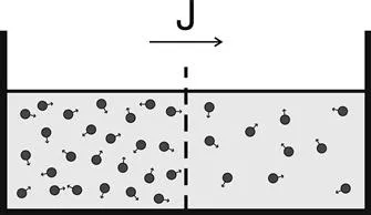
Figure 1.1 According to Fick’s first law, when the specimen contains different regions with different concentrations of molecules, the particles will, on average, tend to move from high concentration regions to low concentration regions leading to a net flux (J).

On a molecular level diffusive mixing results solely from collisions between atoms or molecules in the liquid or gas state. Another interesting feature of diffusion is that it occurs even in thermodynamic equilibrium, for example in a jar of water kept at a constant temperature and pressure. This is quite remarkable because the classical picture of diffusion, as expressed above in Fick’s first law, implies that when the temperature or concentration gradients vanish, there is no net flux. There were many who held that diffusive mixing or energy transfer stopped at this point. We now know that although the net flux vanishes, microscopic motions of molecule still persist; it is just that on average, there is no net molecular flux in equilibrium.

A framework that explains this phenomenon has its origins in the observations of Robert Brown, who is credited with being the first one to report the random motions of pollen grains while studying them under his microscope (Brown, 1828); his observation is illustrated in a cartoon in Figure 1.2. He reported that particles moved randomly without any apparent cause. Brown initially believed that there was some life force that was causing these motions, but disabused himself of this notion when he observed the same fluctuations when studying dust and other dead matter.

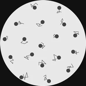
Figure 1.2 Robert Brown, a botanist working on the mechanisms of fertilization in flowering plants, noticed the perpetual motion of pollen grains suspended in water in 1827.

In the early part of the 20th century, Albert Einstein, who was unaware of Brown’s observation and seeking evidence that would undoubtedly imply the existence of atoms, came to the conclusion that (Einstein, 1905; Fürth and Cowper, 1956) “…bodies of microscopically visible size suspended in a liquid will perform movements of such magnitude that they can be easily observed in a microscope”. Einstein used a probabilistic framework to describe the motion of an ensemble of particles undergoing diffusion, which led to a coherent description of diffusion, reconciling the Fickian and Brownian pictures. He introduced the “displacement distribution” for this purpose, which quantifies the fraction of particles that will traverse a certain distance within a particular timeframe, or equivalently, the likelihood that a single given particle will undergo that displacement. For example, in free diffusion the displacement distribution is a Gaussian function whose width is determined by the diffusion coefficient as illustrated in Figure 1.3. Gaussian diffusion will be treated in more detail in Chapter 3, whereas the more general case of non-Gaussianity will be tackled in Chapters 4 and 7.

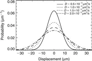
Figure 1.3 The Gaussian displacement distribution plotted for various values of the diffusion coefficient when the diffusion time was taken to be 40 ms. Larger diffusion coefficients lead to broader displacement probabilities suggesting increased diffusional mobility.

Using the displacement distribution concept, Einstein was able to derive an explicit relationship between the mean-squared displacement of the ensemble, characterizing its Brownian motion, and the classical diffusion coefficient, D, appearing in Fick’s law (Einstein, 1905, 1926), given by

(1.2)

where 〈x²〉 is the mean-squared displacement of particles during a diffusion time, Δ, and D is the same classical diffusion coefficient appearing in Fick’s first law above.

At around the same time as Einstein, Smoluchowski (1906) was able to reach the same conclusions using different means. Langevin improved upon Einstein’s description of diffusion for ultra-short timescales in which there are few molecular collisions, but we are not able to probe this regime using MR diffusion measurements in water. Since a particle experiences about 10²¹ collisions every second in typical proton-rich solvents like water (Chandrasekhar, 1943), we generally do not concern ourselves with this correction in diffusion MR.

II Magnetic Resonance and Diffusion

Magnetic resonance provides a unique opportunity to quantify the diffusional characteristics of a wide range of specimens. Because diffusional processes are influenced by the geometrical structure of the environment, MR can be used to probe the structural environment non-invasively. This is particularly important in studies that involve biological samples in which the characteristic length of the boundaries influencing diffusion are typically so small that they cannot be resolved by conventional magnetic resonance imaging (MRI) techniques.

A typical nuclear magnetic resonance (NMR) scan starts with the excitation of the nuclei with a 90 degree radiofrequency (rf) pulse that tilts the magnetization vector into the plane whose normal is along the main magnetic field. The spins subsequently start to precess around the magnetic field – a phenomenon called Larmor precession. The angular frequency of this precession is given by

(1.3)

where B is the magnetic field that the spin is exposed to and γ is the gyromagnetic ratio – a constant specific to the nucleus under examination. In water, the hydrogen nucleus (i.e. the proton) has a gyromagnetic ratio value of approximately 2.68×10⁸ rad/s/tesla. Spins that are initially coherent dephase due to factors such as magnetic field inhomogeneities and dipolar interactions (Abragam, 1961) leading to a decay of the voltage (signal) induced in the receiver.

As proposed by Edwin Hahn (Hahn, 1950), and illustrated in Figure 1.4, the dephasing due to magnetic field inhomogeneities can be reversed through a subsequent application of a 180 degree rf pulse, and the signal is reproduced. In this “spin-echo” experiment, the time between the first rf pulse and formation of the echo is called TE and it is twice the time between the two rf pulses, which...

Table of contents

• Cover image
• Title page
• Table of Contents
• Copyright Page
• Contributors
• Preface
• Foreword
• Section 1: Introduction to Diffusion MRI
• Section 2: Diffusion MRI for Quantitative Measurement
• Section 3: Diffusion MRI for in vivo Neuroanatomy
• Index