Fluid Flow for Chemical Engineers

F. Holland, R. Bragg

• Publisher: Butterworth-Heinemann
• Year: 1995
• ISBN:
  9780080523699
• Edition: 2
• Topic: Technology & Engineering
• Subtopic: Chemical & Biochemical Engineering
• Index: Technology & Engineering

This major new edition of a popular undergraduate text covers topics of interest to chemical engineers taking courses on fluid flow. These topics include non-Newtonian flow, gas-liquid two-phase flow, pumping and mixing. It expands on the explanations of principles given in the first edition and is more self-contained. Two strong features of the first edition were the extensive derivation of equations and worked examples to illustrate calculation procedures. These have been retained. A new extended introductory chapter has been provided to give the student a thorough basis to understand the methods covered in subsequent chapters.

1

Fluids in motion

1.1 Units and dimensions

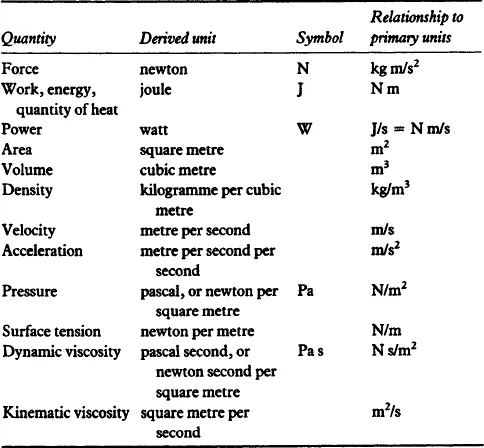
Mass, length and time are commonly used primary units, other units being derived from them. Their dimensions are written as M, L and T respectively. Sometimes force is used as a primary unit. In the Système International d’Unités, commonly known as the SI system of units, the primary units are the kilogramme kg, the metre m, and the second s. A number of derived units are listed in Table 1.1.

Table 1.1

1.2 Description of fluids and fluid flow

1.2.1 Continuum hypothesis

Although gases and liquids consist of molecules, it is possible in most cases to treat them as continuous media for the purposes of fluid flow calculations. On a length scale comparable to the mean free path between collisions, large rapid fluctuations of properties such as the velocity and density occur. However, fluid flow is concerned with the macroscopic scale: the typical length scale of the equipment is many orders of magnitude greater than the mean free path. Even when an instrument is placed in the fluid to measure some property such as the pressure, the measurement is not made at a point—rather, the instrument is sensitive to the properties of a small volume of fluid around its measuring element. Although this measurement volume may be minute compared with the volume of fluid in the equipment, it will generally contain millions of molecules and consequently the instrument measures an average value of the property. In almost all fluid flow problems it is possible to select a measurement volume that is very small compared with the flow field yet contains so many molecules that the properties of individual molecules are averaged out.

It follows from the above facts that fluids can be treated as continuous media with continuous distributions of properties such as the pressure, density, temperature and velocity. Not only does this imply that it is unnecessary to consider the molecular nature of the fluid but also that meaning can be attached to spatial derivatives, such as the pressure gradient dP/dx, allowing the standard tools of mathematical analysis to be used in solving fluid flow problems.

Two examples where the continuum hypothesis may be invalid are low pressure gas flow in which the mean free path may be comparable to a linear dimension of the equipment, and high speed gas flow when large changes of properties occur across a (very thin) shock wave.

1.2.2 Homogeneity and isotropy

Two other simplifications that should be noted are that in most fluid flow problems the fluid is assumed to be homogeneous and isotropic. A homogeneous fluid is one whose properties are the same at all locations and this is usually true for single–phase flow. The flow of gas–liquid mixtures and of solid–fluid mixtures exemplifies heterogeneous flow problems.

A material is isotropic if its properties are the same in all directions. Gases and simple liquids are isotropic but liquids having complex, chain–like molecules, such as polymers, may exhibit different properties in different directions. For example, polymer molecules tend to become partially aligned in a shearing flow.

1.2.3 Steady flow and fully developed flow

Steady processes are ones that do not change with the passage of time. If φ denotes a property of the flowing fluid, for example the pressure or velocity, then for steady conditions

(1.1)

for all properties. This does not imply that the properties are constant: they may vary from location to location but may not change at any fixed position.

Fully developed flow is flow that does not change along the direction of flow. An example of developing and fully developed flow is that which occurs when a fluid flows into and through a pipe or tube. Along most of the length of the pipe, there is a constant velocity profile: there is a maximum at the centre–line and the velocity falls to zero at the pipe wall. In the case of laminar flow of a Newtonian liquid, the fully developed velocity profile has a parabolic shape. Once established, this fully developed profile remains unchanged until the fluid reaches the region of the pipe exit. However, a considerable distance is required for the velocity profile to develop from the fairly uniform velocity distribution at the pipe entrance. This region where the velocity profile is developing is known as the entrance length. Owing to the changes taking place in the developing flow in the entrance length, it exhibits a higher pressure gradient. Developing flow is more difficult to analyse than fully developed flow owing to the variation along the flow direction.

1.2.4 Paths, stre...

Table of contents

• Cover image
• Title page
• Table of Contents
• Copyright
• List of examples
• Preface to the second edition
• Nomenclature
• Chapter 1: Fluids in motion
• Chapter 2: Flow of incompressible Newtonian fluids in pipes and channels
• Chapter 3: Flow of incompressible non-Newtonian fluids in pipes
• Chapter 4: Pumping of liquids
• Chapter 5: Mixing of liquids in tanks
• Chapter 6: Flow of compressible fluids in conduits
• Chapter 7: Gas–liquid two-phase flow
• Chapter 8: Flow measurement
• Chapter 9: Fluid motion in the presence of solid particles
• Chapter 10: Introduction to unsteady flow
• Appendix I: The Navier–Stokes equations
• Appendix II: Further problems
• Answers to problems
• Conversion factors
• Friction factor flow charts
• Index