Geochemical Anomaly and Mineral Prospectivity Mapping in GIS

E.J.M. Carranza

• Publisher: Elsevier Science
• Year: 2008
• ISBN:
  9780080930312
• Topic: Physical Sciences
• Subtopic: Geology & Earth Sciences

Geochemical Anomaly and Mineral Prospectivity Mapping in GIS documents and explains, in three parts, geochemical anomaly and mineral prospectivity mapping by using a geographic information system (GIS). Part I reviews and couples the concepts of (a) mapping geochemical anomalies and mineral prospectivity and (b) spatial data models, management and operations in a GIS. Part II demonstrates GIS-aided and GIS-based techniques for analysis of robust thresholds in mapping of geochemical anomalies. Part III explains GIS-aided and GIS-based techniques for spatial data analysis and geo-information sybthesis for conceptual and predictive modeling of mineral prospectivity. Because methods of geochemical anomaly mapping and mineral potential mapping are highly specialized yet diverse, the book explains only methods in which GIS plays an important role. The book avoids using language and functional organization of particular commercial GIS software, but explains, where necessary, GIS functionality and spatial data structures appropriate to problems in geochemical anomaly mapping and mineral potential mapping. Because GIS-based methods of spatial data analysis and spatial data integration are quantitative, which can be complicated to non-numerate readers, the book simplifies explanations of mathematical concepts and their applications so that the methods demonstrated would be useful to professional geoscientists, to mineral explorationists and to research students in fields that involve analysis and integration of maps or spatial datasets. The book provides adequate illustrations for more thorough explanation of the various concepts.

• Explains GIS functionality and spatial data structures appropriate regardless of the particular GIS software in use
• Simplifies explanation of mathematical concepts and application
• Illustrated for more thorough explanation of concepts

Handbook of Exploration and Environmental Geochemistry 11, Vol. 11, Number Suppl (C), 2009

ISSN: 1874-2734

doi: 10.1016/S1874-2734(09)70005-1

Chapter 1: Predictive Modeling of Mineral Exploration Targets

Introduction

Mineral exploration endeavours to find mineral deposits, especially those with commercially viable concentrations of minerals or metals, for mining purposes. It has four phases, namely (1) area selection, (2) target generation, (3) resource evaluation and (4) reserve definition. Area selection defines permissive regions where mineral deposits of the type sought plausibly exist based on knowledge of environments at or near the surface of the Earth’s crust where the geological processes (e.g., plate tectonics) are or were favourable for mineral deposit formation (Singer, 1993). Target generation demarcates, within permissive regions, prospective areas for further investigations until mineral deposits of interest are discovered based on exploration models for the deposit-type sought and on relevant thematic geoscience (geological, geochemical and geophysical) data sets. Resource evaluation estimates grade and tonnage of specific minerals or metals in discovered mineral deposits based largely on systematic drilling. Reserve definition classifies the various parts of mineral deposits as ore reserves (proved, probable) or mineral resources (measured, indicated, inferred) based on economic and technical feasibility analysis. This volume is concerned with only the target generation phase in mineral exploration.

Target generation is a multi-stage mapping activity from regional-scale to local-scale. Every scale of target generation involves collection, analysis and integration of various thematic geoscience data sets in order to extract pieces of spatial geo-information, namely (a) geological, geochemical and/or geophysical anomalies associated with mineral deposits of the type sought and (b) prospective areas defined by intersections of such anomalies. An example of a geological anomaly is hydrothermal alteration, although it may not necessarily be accompanied by mineral deposits. A geophysical anomaly is a variation from normal background patterns of measured physical properties of the Earth’s upper crust (e.g., magnetism), which can be attributed to localised near-surface or subsurface materials such as metallic mineral deposits. A geochemical anomaly is a departure from the geochemical patterns that are normal for a given area. It can represent either geogenic (i.e., natural) or anthropogenic (i.e., industry-induced) enrichment in one or more elements in Earth materials. In mineral exploration, geochemical anomalies associated with mineral deposits are called significant anomalies, whereas geochemical anomalies associated with other natural processes or anthropogenic processes are called non-significant anomalies. Because not every anomaly is associated, genetically and/or spatially, with mineral deposits of the type sought, intersecting or integrated anomalies of various types are of interest in target generation. The process of analysing and integrating such pieces of spatial geo-information is called predictive modeling. This volume is further concerned with predictive modeling of only geochemical anomalies and prospective areas.

This chapter explains the concepts of (a) predictive modeling, (b) predictive modeling of geochemical anomalies and prospective areas and (c) application of a geographic information system (GIS) in predictive modeling of geochemical anomalies and prospective areas. A GIS consists of computer hardware, computer software, geographically-referenced or spatial data sets and personnel.

What is Predictive Modeling?

To understand the concepts of predictive modeling of geochemical anomalies and prospective areas via applications of GIS, it is imperative to define and understand what model means. The Wiktionary (Wikimedia Foundation, 2007) defines model as “a simplified representation (usually mathematical) used to explain the workings of a real world system or event”. The Oxford English Dictionary (Oxford University Press, 2007) defines model as “a simplified or idealized description or conception of a particular system, situation, or process, often in mathematical terms, that is put forward as a basis for theoretical or empirical understanding, or for calculations, predictions, etc.; a conceptual or mental representation of something”. The Glossary of Geology (American Geological Institute, 2007) defines model as “a working hypothesis or precise simulation, by means of description, statistical data, or analogy, of a phenomenon or process that cannot be observed directly or that is difficult to observe directly. Models may be derived by various methods, e.g. by computer, from stereoscopic photographs, or by scaled experiments”.

Based on the definitions of a model, predictive modeling can be defined as “making descriptions, representations or predictions about an indirectly observable and complex real-world system via (quantitative) analysis of relevant data”. It involves a target variable of interest, which is usually the behaviour (e.g., presence or absence) of an indirectly observable and complex real-world system (e.g., mineralisation), and a number of explanatory or predictor variables or properties that are directly observable or measurable as well as considered to be inter-related with each other and related to that system. Predictive modeling is therefore based on (a) inter-relationships amongst predictor variables, which may reveal patterns related to the target variable and (b) relationships between the target and predictor variables. The latter means that some quantity of data associated directly with the target variable must be available in order to create and to validate a predictive model. A predictive model is a temporal snap-shot of the system of interest, meaning that it embodies the knowledge and/or data sets used at the time of its creation and thus it must be updated whenever new knowledge and/or relevant data sets become available. Therefore, any cartographic representation of an indirectly observable and complex real-world system is a predictive model.

Predictive modeling is relevant to mapping of geochemical anomalies and prospective areas because these real-world systems are complex and indirectly observable. The objective of predictive modeling of geochemical anomalies and/or prospective areas is to represent or map them as discrete spatial entities or geo-objects, i.e., with conceivable boundaries. This entails various forms of data analysis in order to derive and integrate pieces of information that allow description, representation or prediction of geochemical anomalies and/or prospective areas. The term representation or prediction is equivalent to mapping, which embodies results of analyses and interpretations of various relevant geoscience spatial data sets according to hypotheses or propositions about geochemical anomalies and/or prospective areas. Therefore, a map of geochemical anomalies and/or prospective areas is a predictive model of where mineral deposits of interest are likely to exist.

Approaches to predictive modeling

There are two approaches to predictive modeling – induction and deduction. Induction is the process of making generalisations about particular instances in a set of observations or data. A generalisation is derived by studying patterns in a data set. Deduction – the inverse of induction – is the process of confirming particular instances based on a generalisation about patterns in a set of observations or data. The confirmation of particular instances is made by testing a generalisation against every observation or datum. The distinction between induction and deduction can be illustrated via a hypothetical example in Fig. 1-1 (cf. Bonham-Carter, 1994, pp. 180). An initial visual analysis of the distributions of Fe contents in soil vis-à-vis the distributions of lithologic units (Fig. 1-1A), may lead one to hypothesise that soils in areas underlain by basalts have higher Fe contents than soils in areas underlain by other lithologic units. The hypothesis may be supported by a simple linear model of Fe contents generally decaying with distance from the basalt unit (Fig. 1-1B). The map of spatial distributions of Fe contents and the simple linear model may further lead one to make a generalisation that basalts influence Fe contents in soils and that Fe data in soils are useful aids to lithologic mapping. Up to this point, one has performed an induction because a generalisation was made based on particular instances in a set of observations or data. To test the generalisation, because there is always an ‘exception to the rule’, one has to perform deduction. To do so, one may use the simple linear model to predict Fe contents in soil as function of distance to basalt and then map the spatial distributions of residual Fe contents (Fig. 1-1C). The presence of enriched Fe in soils (i.e., positive residuals) in certain parts of the area may lead one to hypothesise that there are unmapped basalt units. Confirmation of this hypothesis requires re-visiting the sample sites (i.e., every particular instance), which could result in updating of the lithologic map (Fig. 1-1C).

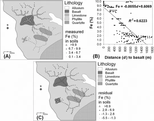
Fig. 1-1 (A) Existing lithologic map and measured Fe (%) contents in ridge-and-spur soil samples. The measured Fe contents in soil generally decrease with distance from the basalt. (B) Best-fit line model for measured Fe contents in soil and distance to the basalt. (C) Updated lithologic map after field investigation of residuals (measured-predicted) of Fe in soil.

Induction and deduction are therefore complementary to each other, such that switching from induction to deduction or vice versa at intermediate steps in predictive modeling could provide better description, understanding and discovery of the system of interest. Thus, despite the approach in the preceding hypothetical example, it is not necessary to initiate predictive modeling with induction. The evolution of scientific knowledge has led to theories or generalisations about dispersion of elements and surface geochemical expressions of mineralisation (Bradshaw, 1975; Kauranne, 1975; Lovering and McCarthy, 1978; Butt and Smith, 1980; Smith, 1987) and genesis of mineral deposits (e.g., Lindgren, 1933; Pirajno, 1992; Evans, 1993; Richards and Tosdal, 2001; Robb, 2004). Therefore, many cases of predictive modeling involved in target generation commence with deduction, although switching to induction may be necessary at intermediate steps until a final predictive model is obtained.

Types of predictive modeling

This section reviews the types of predictive modeling that are relevant to mineral exploration, especially in the target generation phase. There is no generally accepted classification of types of predictive modeling of Earth systems such as geochemical anomalies and prospective areas. However, based on the way inter-predictor relationships and target-predictor relationships are described or represented, two types of predictive modeling – mechanistic and empirical – and hybrids of these two types can be distinguished (cf. Harbaugh and Bonham-Carter, 1970).

Mechanistic modeling applies fundamental or theoretical knowledge of individual predictor variables (i.e., processes) and their interactions in order to predict or understand the target variable of interest. Mechanistic modeling is therefore equivalent to theoretical modeling. Mechanistic modeling relies on mathematical equations to describe the interactions of processes that control the behaviour of system of interest. It applies relevant physical laws and is often based on laboratory studies, field experiments and physical models. Solving the theoretical equations in mechanistic modeling can be complex and require application of generalising or simplifying assumptions (e.g., simplified geometry, homogeneity, idealised initial conditions and boundary conditions). Mechanistic modeling therefore invariably follows a deductive approach. The predictive capability of a mechanistic model can be determined and then improved via probabilistic uncertainty analyses to investigate sensitivity of prediction to one or more predictor variables or assumptions.

There are two sub-types of mechanistic modeling – deterministic and stochastic. Deterministic modeling applies mathematical representations (e.g., differential equations) of the processes that control the behaviour of system of interest. It makes definite predictions of quantities (e.g., metal concentrations) without considering any randomness in the distributions of the variables in the mathematical equations. Stochastic modeling also applies mathematical representations of the processes that control the behaviour of system of interest, but it considers the presence of some random distribution in one or more predictor variables and in the target variable. Stochastic modeling therefore does not result in single estimates of the target variable but a probability distribution of estimates, which is derived from a large number of simulations (stochastic projections), reflecting random distributions in the predictor and target variables. Purely deterministic modeling has been rarely, if not never, used in mineral exploration, except in laboratory studies of mineral deposit formation (e.g., L’Heureux and Katsev, 2006). Purely stochastic modeling is seldom used in the target generation phase of mineral exploration, but it has been applied, however, in the resource estimation and reserve definition phases of mineral exploration (e.g., Sahu, 1982; Harris, 1984; Sahu and Raiker, 1985).

An interesting application of stochastic modeling is where the target variable sought represents fractal geo-objects as a result of stochastic rather than deterministic processes. A fractal geo-object is one which can be fragmented into various parts, and each fragment has similar geometry as the whole geo-object (Mandelbrot, 1983). Geochemical dispersion patterns and spatial distributions of mineral deposits are postulated to be fractals (Bölviken et al., 1992; Agterberg et al., 1993b). Agterberg (2001) and Rantitsch (2001) have demonstrated the utility of stochastic modeling to examine the fractal geometry of geochemical landscapes, as conventional geostatistical methods are not able to do so when the spatial variability of geochemical anomalies exceeds the spatial resolution (i.e., sampling density) of geochemical data sets. Hybrids of stochastic modeling (not based on assumption of fractals) and quantitative empirical modeling (see below) have been applied, however, in mapping of significant geochemical anomalies (e.g., Singer and Kouda, 2001; Agterberg, 2007) and prospective areas (e.g., Agterberg, 1974; Pan et al., 1992; Grunsky et al., 1994).

In contrast to mechanistic modeling, empirical modeling is appropriate when the underlying geochemical and/or physical processes that control the behaviour of the system of interest are insufficiently or indirectly known. Methods for empirical modeling do not take into account interactions of such processes in a mathematical sense as in mechanistic modeling. Instead, they characterise or quantify the influence of one or more of such processes on the behaviour of the system of interest via empirical model equations. Empirical modeling is therefore equivalent to symbolic modeling and generally follows an inductive approach. The equations in empirical modeling are constructed to define relationships between the target variable and a number of predictor variables representing processes in order to describe or symbolise the observed or predicted behaviour of the system of interest. Empirical modeling requires substantial amounts of data of both the target and predictor variables in order to quantify accurately their relationships. In terms of sufficiency of data of the target variable, there are two sub-types of empirical modeling – quantitative and qualitative.

Quantitative empirical modeling is appropriate when data of the target variable are sufficient to obtain, say, statistically significant results. Data of the target variable are usually divided into a training set and a testing set. Based on a training set, relationships between the target and predictor variables are quantified and then used for prediction. Methods for quantitative empirical modeling can be statistical, probabilistic or mathematical. The quality of a quantitative empirical model is described by its goodness-of-fit to data in a training set and its predictive ability against data in a testing set. In mapping of prospective areas, quantitative empirical modeling is also known as data-driven modeling. In contrast, qualitative or heuristic modeling is appropriate when data of the target variable are insufficient or absent. In qualitative modeling, relationships between the target and predictor variables are defined based on expert opinion. Qualitative modeling thus seems to follow a deductive approach. The quality of a qualitative empirical model can be described by its predictive ability against available (albeit insufficient) data of the target variable. In mapping of prospective areas, qualitative empirical modeling is also known as knowledge-driven modeling.

Based on the preceding discussion, further distinctions between mechanistic modeling and empirical modeling can be made as follows. Whereas mechanistic modeling attempts to characterise and understand the fundamental or theoretical processes that control the behaviour of the system of interest, empirical modeling attempts to depict quantitatively the influence of well-understood processes on the behaviour of the system of interest. Therefore, mechanistic modeling strives to derive realistic predictive models, whereas empirical modeling endeavours to derive approximate yet plausible predictive models. Furthermore, mechanistic modeling is dynamic, because it can contain the time variable in the mathematical equations especially in deterministic modeling; whereas empirical modeling usually ignores the time variable and is therefore static. Predictive modeling of geochemical anomali...

Table of contents

• Cover image
• Title page
• Table of Contents
• Edited by
• Copyright
• Editor’s Foreword
• Preface
• Chapter 1: Predictive Modeling of Mineral Exploration Targets
• Chapter 2: Spatial Data Models, Management and Operations
• Chapter 3: Exploratory Analysis of Geochemical Anomalies
• Chapter 4: Fractal Analysis of Geochemical Anomalies
• Chapter 5: Catchment Basin Analysis of Stream Sediment Anomalies
• Chapter 6: Analysis of Geologic Controls on Mineral Occurrence
• Chapter 7: Knowledge-Driven Modeling of Mineral Prospectivity
• Chapter 8: Data-Driven Modeling of Mineral Prospectivity
• References
• Online Sources
• Author Index
• Subject Index