Electric Motors and Drives

Fundamentals, Types and Applications

Austin Hughes, Bill Drury

• Publisher: Newnes
• Year: 2013
• ISBN:
  9780080993683
• Edition: 4
• Topic: Technology & Engineering
• Subtopic: Electrical Engineering & Telecommunications
• Index: Technology & Engineering

Electric Motors and Drives is intended for non-specialist users of electric motors and drives, filling the gap between maths- and theory-based academic textbooks and the more prosaic 'handbooks', which provide useful detail but little opportunity for the development of real insight and understanding. The book explores all of the widely-used modern types of motor and drive, including conventional and brushless D.C., induction motors and servo drives, providing readers with the knowledge to select the right technology for a given job.The third edition includes additional diagrams and worked examples throughout. New topics include digital interfacing and control of drives, direct torque control of induction motors and current-fed operation in DC drives. The material on brushless servomotors has also been expanded.Austin Hughes' approach, using a minimum of maths, has established Electric Motors and Drives as a leading guide for electrical engineers and mechanical engineers, and the key to a complex subject for a wider readership, including technicians, managers and students.

• Acquire knowledge of and understanding of the capabilities and limitations of motors and drives without struggling through unnecessary maths and theory
• Updated material on the latest and most widely-used modern motors and drives, including brushless servomotors
• New edition includes additional diagrams and worked examples throughout

Chapter One

Electric Motors – The Basics

1. Introduction

Electric motors are so much a part of everyday life that we seldom give them a second thought. When we switch on an ancient electric drill, for example, we confidently expect it to run rapidly up to the correct speed, and we don’t question how it knows what speed to run at, or how it is that once enough energy has been drawn from the supply to bring it up to speed, the power drawn falls to a very low level. When we put the drill to work it draws more power, and, when we finish, the power drawn from the mains reduces automatically, without intervention on our part.

The humble motor, consisting of nothing more than an arrangement of copper coils and steel laminations, is clearly rather a clever energy converter, which warrants serious consideration. By gaining a basic understanding of how the motor works, we will be able to appreciate its potential and its limitations, and (in later chapters) see how its already remarkable performance is dramatically enhanced by the addition of external electronic controls.

This chapter deals with the basic mechanisms of motor operation, so readers who are already familiar with such matters as magnetic flux, magnetic and electric circuits, torque, and motional e.m.f. can probably afford to skim over much of it. In the course of the discussion, however, several very important general principles and guidelines emerge. These apply to all types of motor and are summarized in section 9. Experience shows that anyone who has a good grasp of these basic principles will be well equipped to weigh the pros and cons of the different types of motor, so all readers are urged to absorb them before tackling other parts of the book.

2. Producing Rotation

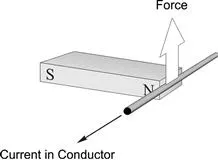
Nearly all motors exploit the force which is exerted on a current-carrying conductor placed in a magnetic field. The force can be demonstrated by placing a bar magnet near a wire carrying current (Figure 1.1), but anyone trying the experiment will probably be disappointed to discover how feeble the force is, and will doubtless be left wondering how such an unpromising effect can be used to make effective motors.

Figure 1.1 Mechanical force produced on a current-carrying wire in a magnetic field.

We will see that in order to make the most of the mechanism, we need to arrange for there to be a very strong magnetic field, and for it to interact with many conductors, each carrying as much current as possible. We will also see later that although the magnetic field (or ‘excitation’) is essential to the working of the motor, it acts only as a catalyst, and all of the mechanical output power comes from the electrical supply to the conductors on which the force is developed.

It will emerge later that in some motors the parts of the machine responsible for the excitation and for the energy-converting functions are distinct and self-evident. In the d.c. motor, for example, the excitation is provided either by permanent magnets or by field coils wrapped around clearly defined projecting field poles on the stationary part, while the conductors on which force is developed are on the rotor and supplied with current via sliding brushes. In many motors, however, there is no such clear-cut physical distinction between the ‘excitation’ and the ‘energy-converting’ parts of the machine, and a single stationary winding serves both purposes. Nevertheless, we will find that identifying and separating the excitation and energy-converting functions is always helpful in understanding how motors of all types operate.

Returning to the matter of force on a single conductor, we will look first at what determines the magnitude and direction of the force, before turning to ways in which the mechanism is exploited to produce rotation. The concept of the magnetic circuit will have to be explored, since this is central to understanding why motors have the shapes they do. Before that, a brief introduction to the magnetic field and magnetic flux and flux density is included for those who are not already familiar with the ideas involved.

2.1 Magnetic field and magnetic flux

When a current-carrying conductor is placed in a magnetic field, it experiences a force. Experiment shows that the magnitude of the force depends directly on the current in the wire and the strength of the magnetic field, and that the force is greatest when the magnetic field is perpendicular to the conductor.

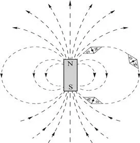
In the set-up shown in Figure 1.1, the source of the magnetic field is a bar magnet, which produces a magnetic field as shown in Figure 1.2.

Figure 1.2 Magnetic flux lines produced by a permanent magnet.

The notion of a ‘magnetic field’ surrounding a magnet is an abstract idea that helps us to come to grips with the mysterious phenomenon of magnetism: it not only provides us with a convenient pictorial way of visualizing the directional effects, but it also allows us to quantify the ‘strength’ of the magnetism and hence permits us to predict the various effects produced by it.

The dotted lines in Figure 1.2 are referred to as magnetic flux lines, or simply flux lines. They indicate the direction along which iron filings (or small steel pins) would align themselves when placed in the field of the bar magnet. Steel pins have no initial magnetic field of their own, so there is no reason why one end or the other of the pins should point to a particular pole of the bar magnet.

However, when we put a compass needle (which is itself a permanent magnet) in the field we find that it aligns itself as shown in Figure 1.2. In the upper half of the figure, the S end of the diamond-shaped compass settles closest to the N pole of the magnet, while in the lower half of the figure, the N end of the compass seeks the S of the magnet. This immediately suggests that there is a direction associated with the lines of flux, as shown by the arrows on the flux lines, which conventionally are taken as positively directed from the N to the S pole of the bar magnet.

The sketch in Figure 1.2 might suggest that there is a ‘source’ near the top of the bar magnet, from which flux lines emanate before making their way to a corresponding ‘sink’ at the bottom. However, if we were to look at the flux lines inside the magnet, we would find that they were continuous, with no ‘start’ or ‘finish’. (In Figure 1.2 the internal flux lines have been omitted for the sake of clarity, but a very similar field pattern is produced by a circular coil of wire carrying a direct current – see Figure 1.7 where the continuity of the flux lines is clear.) Magnetic flux lines always form closed paths, as we will see when we look at the ‘magnetic circuit’, and we draw a parallel with the electric circuit, in which the current is also a continuous quantity. (There must be a ‘cause’ of the magnetic flux, of course, and in a permanent magnet this is usually pictured in terms of atomic-level circulating currents within the magnet material. Fortunately, discussion at this physical level is not necessary for our purposes.)

2.2 Magnetic flux density

As well as showing direction, flux plots convey information about the intensity of the magnetic field. To achieve this, we introduce the idea that between every pair of flux lines (and for a given depth into the paper) there is the same ‘quantity’ of magnetic flux. Some people have no difficulty with such a concept, while others find that the notion of quantifying something so abstract represents a serious intellectual challenge. But whether the approach seems obvious or not, there is no denying the practical utility of quantifying the mysterious stuff we call magnetic flux, and it leads us next to the very important idea of magnetic flux density (B).

When the flux lines are close together, the ‘tube’ of flux is squashed into a smaller space, whereas when the lines are further apart the same tube of flux has more breathing space. The flux density (B) is simply the flux in the ‘tube’ (

) divided by the cross-sectional area (A) of the tube, i.e.

(1.1)

The flux density is a vector quantity, and is therefore often written in bold type: its magnitude is given by equation (1.1), and its direction is that of the prevailing flux lines at each point. Near the top of the magnet in Figure 1.2, for example, the flux density will be large (because the flux is squashed into a small area), and pointing upwards, whereas on the equator and far out from the body of the magnet the flux density will be small and directed downwards.

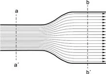
We will see later that in order to create high flux densities in motors, the flux spends most of its life inside well-defined ‘magnetic circuits’ made of iron or steel, within which the flux lines spread out uniformly to take full advantage of the available area. In the case shown in Figure 1.3, for example, the cross-sectional area of the iron at bb′ is twice that at aa′, but the flux is constant so the flux density at bb′ is half that at aa′.

Figure 1.3 Magnetic flux lines inside part of an iron magnetic circuit.

It remains to specify units for quantity of flux, and flux density. In the SI system, the unit of magnetic flux is the weber (Wb). If one weber of flux is distributed uniformly across an area of one square meter perpendicular to the flux, the flux density is clearly one weber per square meter (Wb/m²). This was the unit of B until about 50 years ago, when it was decided that one weber per square meter would...

Table of contents

• Cover image
• Title page
• Table of Contents
• Copyright
• Preface
• Chapter One. Electric Motors – The Basics
• Chapter Two. Introduction to Power Electronic Converters for Motor Drives
• Chapter Three. Conventional D.C. Motors
• Chapter Four. D.C. Motor Drives
• Chapter Five. Induction Motors – Rotating Field, Slip and Torque
• Chapter Six. Induction Motors – Operation from 50/60Hz Supply
• Chapter Seven. Variable Frequency Operation of Induction Motors
• Chapter Eight. Inverter-fed Induction Motor Drives
• Chapter Nine. Synchronous and Brushless Permanent Magnet Machines and Drives
• Chapter Ten. Stepping and Switched-reluctance Motors
• Chapter Eleven. Motor/Drive Selection
• Appendix One. Introduction to Closed-loop Control
• Appendix Two. Induction Motor Equivalent Circuit
• Further Reading
• Index
• Color Plates