Molten Salts Chemistry

From Lab to Applications

Frederic Lantelme, Henri Groult

• Publisher: Elsevier
• Year: 2013
• ISBN:
  9780124017221
• Topic: Physical Sciences
• Subtopic: Industrial & Technical Chemistry

Molten salts and fused media provide the key properties and the theory of molten salts, as well as aspects of fused salts chemistry, helping you generate new ideas and applications for fused salts. Molten Salts Chemistry: From Lab to Applications examines how the electrical and thermal properties of molten salts, and generally low vapour pressure are well adapted to high temperature chemistry, enabling fast reaction rates. It also explains how their ability to dissolve many inorganic compounds such as oxides, nitrides, carbides and other salts make molten salts ideal as solvents in electrometallurgy, metal coating, treatment of by-products and energy conversion.This book also reviews newer applications of molten salts including materials for energy storage such as carbon nano-particles for efficient super capacitors, high capacity molten salt batteries and for heat transport and storage in solar plants. In addition, owing to their high thermal stability, they are considered as ideal candidates for the development of safer nuclear reactors and for the treatment of nuclear waste, especially to separate actinides from lanthanides by electrorefining.

• Explains the theory and properties of molten salts to help scientists understand these unique liquids
• Provides an ideal introduction to this expanding field
• Illustrated text with key real-life applications of molten salts in synthesis, energy, nuclear, and metal extraction

1

Modeling of Molten Salts

M. Salanne^*, C. Simon^*, P. Turq^*, N. Ohtori^† and P.A. Madden^‡, ^*UPMC Univ Paris 06, CNRS, ESPCI, UMR 7195, Laboratoire PECSA, Paris, France, ^†Graduate School of Science and Technology, Niigata University, Niigata, Japan, ^‡Department of Materials, University of Oxford, Oxford, United Kingdom

Abstract

In recent years, molecular modeling has become an indispensable tool for studying the structure and dynamics of molten salts. In this chapter, we first provide a short description of the state-of-the-art models and methods used for modeling molten salts at the atomic scale. In particular, we discuss the importance of polarization effects for obtaining accurate results. We then give some examples of the structure of several molten salts, as yielded by the simulations. We finish by describing how the transport properties, which encompass the diffusion coefficients, electrical conductivities, viscosities, and thermal conductivities, are computed. By comparing the values given by the simulations to reference experimental data, we show that this technique can now be considered as highly predictive.

KeyWords

molten salts; molecular dynamics; polarizable ion model; transport properties; structure

Acknowledgment

Part of the research leading to these results has received funding from the European Community’s Seventh Framework Programme under Grant agreement 249696 EVOL.

1.1 Introduction

Among the large array of techniques, which are devoted to the study of liquid matter, molecular simulations appear as a method of choice [1]. They provide an atomic-scale description of the systems and are therefore used both for interpreting existing experimental data and for predicting unknown properties. In the case of molten salts, this ability is crucial. Indeed, due to the high temperatures and sometimes due to the use of hazardous or radioactive species, experiments in these media are expensive and difficult to realize, if not impossible. Simulation is then an alternative method which allows a wide range of thermodynamic (e.g., temperature) and composition ranges to be spanned for a minimal cost.

The most important ingredient of these molecular simulations is the treatment of interatomic interactions. In the future, it is foreseen that all of them will be calculated at the ab initio level, i.e., by taking explicitly into accounts the electronic degrees of freedom [2], but this is not possible yet for our systems of interest. The most accurate alternative consists in using physically motivated model potentials for the interactions, in which additional degrees of freedom provide a “cartoon” of the response of the electronic structure of the ions to their changing coordination environments, allowing for a compact representation of many-body contributions (e.g., polarization) to the interaction energy [3]. Such potentials are erroneously termed “empirical,” although it is only appropriate when experimental information is used in the parameterization procedure. In molten salts, it is possible to obtain the potential parameters by fitting the predicted forces and multipoles to a large body of information generated from ab initio calculations [4–6].

Of course it is not because a calculation is entirely based on first principles that it provides the correct answer. Any method involves some more-or-less controlled approximations [7], and real systems often involve small impurities, interfaces with vessel furnaces, etc., which are not included in the simulations. Testing the simulations on a set of reliable data is compulsory. As soon as this step has successfully been taken, it is possible to use them in a predictive way. The properties of interest are usually the structure of the melts along with their enthalpy of mixing, heat capacity, and density (i.e., “static” properties) or their diffusion coefficients (one for each species), electrical conductivity, viscosity, and thermal conductivity (“transport” or “dynamic” properties). The list of known quantities varies importantly from one system to another, and molecular simulations are techniques of choice for (i) filling the gaps in the databases and (ii) interpreting the data and linking them one with each other (e.g., linking physical properties of the melt with its structure).

This chapter is organized as follows: In a first section, we will provide a brief summary of the principal methods for performing molecular simulation and of the models which are widely used for simulating molten salts. Then we will provide a state-of-the-art picture of molten salts in terms of structural, static, and dynamic properties. In each of these sections, the basic methodological aspects for extracting the useful information will be explained and a few selected examples will be provided. In the conclusion, future directions for the modeling of molten salts will be proposed.

1.2 Methods and Models

1.2.1 Molecular Dynamics Simulations

Molecular dynamics is a widespread computational technique in which systems are simulated at the atomic scale [1]. In the case of liquids, a simulation cell typically contains 100-10,000 atoms (even more for complex systems), and periodic boundary conditions are used; an example is shown in Figure 1.1 for molten LiF-KF (the lines correspond to the simulation cell limits, at which the periodic boundary conditions are applied). A trajectory of several nanoseconds is then calculated by numerically solving Newton’s equation of motion

(1.1)

for each atom i of position rⁱ and mass mⁱ, in an iterative way. In Equation (1.1), the total force Fⁱ which is acting on the atom derives from the interaction potential, which is defined in the framework of a given model. The models used in the case of molten salts are described in the following. It is worth noting that several statistical mechanics ensembles can be used for simulating a system. In the simplest case, the number of atoms N, the volume of the simulation cell V, and the total energy of the system E are kept fixed (microcanonical ensemble or NVE ensemble). When the system is at the thermodynamic equilibrium, the temperature T and pressure P then fluctuate around an average value. It is nevertheless often very useful to control the temperature by adding a thermostat; then the total energy is no more constant and the system is simulated in the canonical ensemble (or NVT ensemble). This is what has been done in most of the results presented here. Finally, one can also control the pressure, in which case the volume is allowed to fluctuate. Such simulations, performed in the NPT ensemble, are mainly used for determining the equation of state and the constant pressure heat capacity of the system.

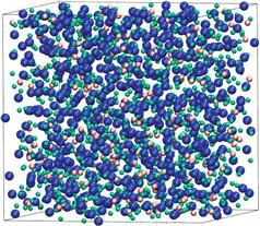
Figure 1.1 Typical simulation cell (equimolar LiF-KF mixture). Ions are shown as spheres, while the lines represent the limits of the cell, where periodic boundary conditions are applied.

1.2.2 The Rigid Ion Model

In a first approximation, ions in a molten salt can be represented as a set of charged spheres with a rigid electron density [8,9]. In such a rigid ion model (RIM), the interaction potential is the sum of three terms:

The first one accounts for the Coulombic interactions:

(1.2)

In this equation, qⁱ is the formal charge carried by the ion i and r^ij is the interatomic distance between i and another ion j. This term is long-ranged and special care must be taken when doing the simulation; the Ewald summation method is generally used [1,10].

The second term is due to the overlap repulsion between the electronic clouds, it reads

(1.3)

where A and a are adjustable parameters for each ionic species pair. It is much shorter-ranged than the Coulombic one and will control the minimal distance at which oppositely charged ions can approach one from each other.

The last term, the dispersion, arises from correlated fluctuations of the electrons; it is always attractive and it takes the form

(1.4)

where C₆ and C₈ are the dipole-dipole (dipole-quadrupole) dispersion coefficients and f_n (n = 6 or 8) are functions that can be introduced to describe the short-range ...

Table of contents

• Cover image
• Title page
• Table of Contents
• Copyright
• Contributors
• Preface
• 1. Modeling of Molten Salts
• 2. Raman Spectroscopy and Pulsed Neutron Diffraction of Molten Salt Mixtures Containing Rare-Earth Trichlorides: Trial Approaches from Fundamentals to Pyrochemical Reprocessing
• 3. In Situ Spectroscopy in Molten Fluoride Salts
• 4. Thermodynamic Calculations of Molten-Salt Reactor Fuel Systems
• 5. Ionic Transport in Molten Salts
• 6. Salt Bath Thermal Treating and Nitriding
• 7. Catalysis in Molten Ionic Media
• 8. The Ability of Molten Carbonate for Gas Cleaning of Biomass Gasification
• 9. Inert Anode Development for High-Temperature Molten Salts
• 10. Boron-Doped Diamond Electrodes in Molten Chloride Systems
• 11. NF3 Production from Electrolysis in Molten Fluorides
• 12. Corrosion in Molten Salts
• 13. Plasma-Induced Discharge Electrolysis for Nanoparticle Production
• 14. Electrochemical Formation of Rare Earth-Nickel Alloys
• 15. Electrochemical Synthesis of Novel Niobium and Tantalum Compounds in Molten Salts
• 16. Preparation of Carbonaceous Materials in Fused Carbonate Salts: Applications to Electrochemical Storages Devices
• 17. Molten Carbonates from Fuel Cells to New Energy Devices
• 18. Synthesis and Li+ Ion Exchange in Molten Salts of Novel Hollandite-Type Ky(Mn1−xCox)O2·zH2O Nanofiber for Lithium Battery Electrodes
• 19. Hybrid Molten Carbonate/Solid Oxide Direct Carbon Fuel Cells
• 20. High-Temperature Molten Salts for Solar Power Application
• 21. The Sodium Metal Halide (ZEBRA) Battery: An Example of Inorganic Molten Salt Electrolyte Battery
• 22. Hydrogen Storage and Transportation System through Lithium Hydride Using Molten Salt Technology
• 23. Nuclear Energy Based on Thorium Molten Salt
• 24. Molten Salts for Nuclear Applications
• 25. Lanthanides Extraction Processes in Molten Fluoride Media
• 26. Development of Pyrochemical Separation Processes for Recovery of Actinides from Spent Nuclear Fuel in Molten LiCl-KCl
• Index