Microwave/RF Applicators and Probes for Material Heating, Sensing, and Plasma Generation

A Design Guide

Mehrdad Mehdizadeh

• Publisher: William Andrew
• Year: 2009
• ISBN:
  9780815519867
• Topic: Tecnología e ingeniería
• Subtopic: Ingeniería general

Interactions of electromagnetic fields with materials at high frequencies have given rise to a vast array of practical applications in industry, science, medicine, and consumer markets. Applicators or probes, which are the front end of these systems, provide the field that interacts with the material. This book takes an integrated approach to the area of high frequency applicators and probes for material interactions, providing a toolkit for those who design these devices. Particular attention is given to real-world applications and the latest developments in the area.

Mathematical methods are provided as design tools, and are often simplified via curve-fitting techniques that are particularly usable by handheld calculators. Useful equations and numerically solved examples, using situations encountered in practice, are supplied. Above all, this volume is a comprehensive and useful reference where the reader can find design rules and principles of high frequency applicators and probes for material processing and sensing applications. Electronic and electrical R&D engineers, physicists, university professors and students will all find this book a valuable reference.

Mehrdad Mehdizadeh is with the DuPont Company, Engineering Research & Technology Division in Wilmington, Delaware. His areas of expertise include high frequency hardware and electromagnetic methods of processing, sensing, and characterization of materials. His work and innovation in industrial, scientific, and medical applications of radio frequency and microwaves has resulted in 19 US patents and a number of publications. He earned his Ph.D. and M.S. from Marquette University (1983, 1980), and a B.S. from Sharif University of Technology (1977), all in electrical engineering. Dr. Mehdizadeh is a Senior Member of the Institute of Electrical and Electronic Engineers (IEEE ), Sigma Xi (Scientific Research Society), the International Microwave Power Institute (IMPI ), and a voting member of IEEE Standard Association.

• Books in this area are usually theoretical; this book provides practical information for those who actually intend to design a system
• Features real world and numerically solved examples, and curve-fitted simple equations to replace complex equations provided in typical texts
• Author is a voting member of IEEE Standards Association

Chapter 1 The Impact of Fields on Materials at RF/Microwave Frequencies

Introduction

Field interaction with materials is a vast area of science, and a large body of literature is devoted to it. High-frequency applicators and probes operate in a relatively small, but important, part of the electromagnetic spectrum. This chapter serves as a brief background on electromagnetic and material topics related to the scope of this book. Furthermore, a number of definitions, concepts, and equations are reviewed that are referred to in other chapters. For a more extensive treatment of electromagnetic principles and material properties, the interested reader can consult many excellent sources, both in print and online [1–4], in this area.

Knowledge of field–material interactions is critical to the design of the high-frequency applicators, because the electrical properties of the material of interest will become a part of the device’s functioning. This fact is a unique feature of these devices, which sets them apart. For example, in the design of a conventional furnace, it is of little importance what material is to be heated, but the dielectric properties of a material being processed by a microwave applicator are of great importance in the design of the device.

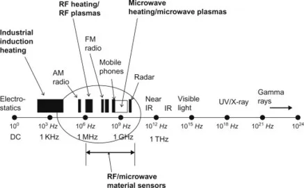
The electromagnetic spectrum is shown in Figure 1.1, and the frequency bands of interest in this book are highlighted. This is a region in the spectrum covering a frequency range typically known as RF, through microwave and into millimeter wave (a few megahertz to tens of gigahertz). This general part of the electromagnetic spectrum happens to be where most wireless telecommunication devices are also housed. The major categories of applications covered in this book, together with their frequency ranges, are noted in Figure 1.1.

Figure 1.1 The electromagnetic spectrum and its usage at various frequencies.

1.1 High-frequency Fields Imposed on Uniform Materials

1.1.1 The wave equations and materials

The essential role of material properties in electromagnetics is readily evident in two of the four Maxwell equations that govern the relationships between electric field vector

and magnetic field vector

:

((1.1))

((1.2))

The three basic material properties σ, ε, and μ are called conductivity, permittivity, and permeability respectively. The above two equations, which are called Ampere’s law and Faraday’s law, relate time variations of one field to spatial variations of the other. In other words, they state that time-varying electric fields induce magnetic fields, and time-varying magnetic fields induce electric fields. The only exception to time-varying requirement is the term in Eq. (1.1), which means in the presence of mobile electric charges (free electrons in conductors), even a non-time-varying electric field can give rise to a magnetic field. This principle is the basis of all direct current (DC) electricity. The converse, however, is not true. Since there are no known magnetic charges, a time-varying electric field cannot exist without an accompanying magnetic field.

Further examination of Ampere’s and Faraday’s laws suggests that the ratio between the intensities of electric magnetic fields in time and space are set by surrounding material properties. Even a vacuum has permittivity and permeability, but not conductivity, since there are no free charges in a vacuum.

The subject of applicators and probes covered in this book is considered using steady-state time-varying systems throughout, which means the time variations of fields as shown in the right-hand sides of Eqs (1.1) and (1.2) are sinusoidal. This fact greatly simplifies relationships between electric and magnetic fields in steady-state systems. Instead of instantaneous values of fields, only the amplitudes of the fields along with the operating frequency need to be considered. In steady state, Eqs (1.1) and (1.2) become:

((1.3))

((1.4))

where at the operating frequency f (in Hz), ω = 2πf is the angular frequency and

is the complex operator. For the rest of this book, unless stated otherwise, the electric field and magnetic fields mentioned are either magnitudes of the steady-state values, or the root mean square (RMS) value, which is a time average of a sine wave.

For solving practical problems involving boundary conditions, combining Eqs (1.3) and (1.4) yields the wave equations in phasor form [5]:

((1.5))

((1.6))

where the operator is called Laplacian, and k is the wave number where:

((1.7))

The angular frequency is ω = 2πf in radians/second (rad/s) and f is the operating frequency in Hz. Note that permittivity, ε in farads/meter (F/m), and magnetic permeability, μ in henries/meter (H/m), in general, are complex quantities, as we will examine later. Their values in free space, however, are ε ₀ = 8.85 × 10⁻¹² F/m and μ ₀ = 4π × 10⁻⁷ H/m.

The wave equations (1.5) and (1.6) are better suited for solving practical boundary value problems such as those in appl...

Table of contents

• Cover
• Title Page
• Copyright
• Dedication
• Table of Contents
• Preface
• Acknowledgement
• Chapter 1: The Impact of Fields on Materials at RF/Microwave Frequencies
• Chapter 2: Fundamentals of Field Applicators and Probes at RF and Microwave Frequencies
• Chapter 3: Electric Field (Capacitive) Applicators/Probes
• Chapter 4: Single-mode Microwave Cavities for Material Processing and Sensing
• Chapter 5: Microwave Multimode Cavities for Material Heating
• Chapter 6: Applicators and Probes Based on the Open End of Microwave Transmission Lines
• Chapter 7: Magnetic Field and Inductive Applicators and Probes at High Frequencies
• Chapter 8: RF/Microwave Applicators and Systems for Joining and Bonding of Materials
• Chapter 9: Design Considerations for Applicators in Continuous-flow Microwave/RF Processing
• Appendices
• Index