Introduction to Groundwater Modeling

Finite Difference and Finite Element Methods

Herbert F. Wang, Mary P. Anderson

• Publisher: Academic Press
• Year: 1995
• Print ISBN: 9780127345857
• eBook ISBN: 9780080571942
• Topic: Physical Sciences
• Subtopic: Geology & Earth Sciences

The dramatic advances in the efficiency of digital computers during the past decade have provided hydrologists with a powerful tool for numerical modeling of groundwater systems. Introduction to Groundwater Modeling presents a broad, comprehensive overview of the fundamental concepts and applications of computerized groundwater modeling.The book covers both finite difference and finite element methods and includes practical sample programs that demonstrate theoretical points described in the text. Each chapter is followed by problems, notes, and references to additional information. This volume will be indispensable to students in introductory groundwater modeling courses as well as to groundwater professionals wishing to gain a complete introduction to this vital subject.- Systematic exposition of the basic ideas and results of Hilbert space theory and functional analysis- Great variety of applications that are not available in comparable books- Different approach to the Lebesgue integral, which makes the theory easier, more intuitive, and more accessible to undergraduate students

Chapter 1. Introduction

1.1. MODELS

A model is a tool designed to represent a simplified version of reality. Given this broad definition of a model, it is evident that we all use models in our everyday lives. For example, a road map is a way of representing a complex array of roads in a symbolic form so that it is possible to test various routes on the map rather than by trial and error while driving a car. A road map could be considered a kind of model (Lehr, 1979) because it is a way of representing reality in a simplified form. Similarly, groundwater models are also representations of reality and, if properly constructed, can be valuable predictive tools for management of groundwater resources. For example, using a groundwater model, it is possible to test various management schemes and to predict the effects of certain actions. Of course, the validity of the predictions will depend on how well the model approximates field conditions. Good field data are essential when using a model for predictive purposes. However, an attempt to model a system with inadequate field data can also be instructive as it may serve to identify those areas where detailed field data are critical to the success of the model. In this way, a model can help guide data collection activities.

Types of Groundwater Models

Several types of models have been used to study groundwater flow systems. They can be divided into three, broad categories (Prickett, 1975): sand tank models, analog models, including viscous fluid models and electrical models, and mathematical models, including analytical and numerical models. A sand tank model consists of a tank filled with ah unconsolidated porous medium through which water is induced to flow. A major drawback of sand tank models is the problem of scaling down a field situation to the dimensions of a laboratory model. Phenomena measured at the scale of a sand tank model are often different from conditions observed in the field, and conclusions drawn from such models may need to be qualified when translated to a field situation.

As we shall see later in the book, the flow of groundwater can be described by differential equations derived from basic principles of physics. Other processes, such as the flow of electrical current through a resistive medium or the flow of heat through a solid, also operate under similar physical principles. In other words, these systems are analogous to the groundwater system. The two types of analogs used most frequently in groundwater modeling are viscous fluid analog models and electrical analog models.

Viscous fluid models are known as Hele–Shaw or parallel plate models because a fluid more viscous than water (for example, oil) is made to flow between two closely spaced parallel plates, which may be oriented either vertically or horizontally. Electrical analog models were widely used in the 1950s before high-speed digital computers became available. These models consist of boards wired with electrical networks of resistors and capacitors. They work according to the principle that the flow of groundwater is analogous to the flow of electricity. This analogy is expressed in the mathematical similarity between Darcy's law for groundwater flow and Ohm's law for the flow of electricity. Changes in voltage in an electrical analog model are analogous to changes in groundwater head. A drawback of an electrical analog model is that each one is designed for a unique aquifer system. When a different aquifer is to be studied, an entirely new electrical analog model must be built.

A mathematical model consists of a set of differential equations that are known to govern the flow of groundwater. Mathematical models of groundwater flow have been in use since the late 1800s. The reliability of predictions using a groundwater model depends on how well the model approximates the field situation. Simplifying assumptions must always be made in order to construct a model because the field situations are too complicated to be simulated exactly. Usually the assumptions necessary to solve a mathematical model analytically are fairly restrictive. For example, many analytical solutions require that the medium be homogeneous and isotropic. To deal with more realistic situations, it is usually necessary to solve the mathematical model approximately using numerical techniques. Since the 1960s, when high-speed digital computers became widely available, numerical models have been the favored type of model for studying groundwater. The subject of this book is the use of numerical methods to solve mathematical models that simulate groundwater flow and contaminant transport.

We consider two types of models—finite difference models (Chapter 2, Chapter 3, Chapter 4 and Chapter 5) and finite element models (Chapter 6, Chapter 7 and Chapter 8). In either case, a system of nodal points is superimposed over the problem domain. For example, consider the problem shown in Figure 1.1. The problem domain consists of an aquifer bounded on one side by a river (Figure 1.1a). The aquifer is recharged areally by precipitation, but there is no horizontal flow out of or into the aquifer except along the river. Two finite difference representations of the problem domain are illustrated in Figures 1.1b and 1.1c and a finite element representation is shown in Figure 1.1d.

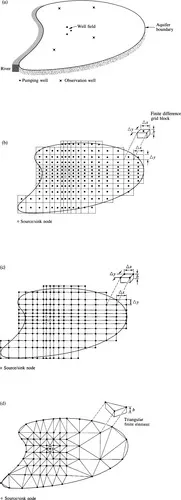Figure 1.1 Finite difference and finite element representations of an aquifer region. (a) Map view of aquifer sho...

Table of contents

• Cover image
• Table of Contents
• Front matter
• Copyright
• Preface
• Chapter 1. Introduction
• Chapter 2. Finite Differences
• Chapter 3. Finite Differences
• Chapter 4. Finite Differences
• Chapter 5. Other Solution Methods
• Chapter 6. Finite Elements
• Chapter 7. Finite Elements
• Chapter 8. Advective-Dispersive Transport
• Concluding Remarks
• Appendix A. Anisotropy and Tensors
• Appendix B. Variational Method
• Appendix C. Isoparametric Quadrilateral Elements
• Appendix D. Analogies
• Glossary of Symbols
• References
• Index