Nanofluidics and Microfluidics

Systems and Applications

Shaurya Prakash, Junghoon Yeom

• Publisher: William Andrew
• Year: 2014
• ISBN:
  9781437744705
• Topic: Technology & Engineering
• Subtopic: Mechanical Engineering
• Index: Technology & Engineering

To provide an interdisciplinary readership with the necessary toolkit to work with micro- and nanofluidics, this book provides basic theory, fundamentals of microfabrication, advanced fabrication methods, device characterization methods and detailed examples of applications of nanofluidics devices and systems. Case studies describing fabrication of complex micro- and nanoscale systems help the reader gain a practical understanding of developing and fabricating such systems. The resulting work covers the fundamentals, processes and applied challenges of functional engineered nanofluidic systems for a variety of different applications, including discussions of lab-on-chip, bio-related applications and emerging technologies for energy and environmental engineering.

• The fundamentals of micro- and nanofluidic systems and micro- and nanofabrication techniques provide readers from a variety of academic backgrounds with the understanding required to develop new systems and applications.
• Case studies introduce and illustrate state-of-the-art applications across areas, including lab-on-chip, energy and bio-based applications.
• Prakash and Yeom provide readers with an essential toolkit to take micro- and nanofluidic applications out of the research lab and into commercial and laboratory applications.

Chapter 1

Introduction

This chapter provides a basic introduction to the concept of microfluidic and nanofluidic (μ-Nafl) systems and presents a layout of the book. The chapter opens with a general definition of μ-Nafl systems. The main theme for the book is structured around the idea of “systems.” The context for each type of system is discussed throughout the book. Surface-area-to-volume (SA/V) ratio is stated as an identifying feature of all μ-Nafl systems. A figure depicting interplay between critical length scales and device volumes driving several applications for μ-Nafl systems is presented. Finally, the chapter concludes by giving direction for future perspective of μ-Nafl systems.

Keywords

Microfluidic and nanofluidic systems; surface-area-to-volume ratio; critical length scales; systems; device volume; future perspective

Chapter outline

1.1 Length scales

1.2 Scope and layout of the book

1.3 Future outlook

References

Select bibliography

1.1 Length scales

Microfluidic and nanofluidic (μ-Nafl) systems are defined as systems with functional components with operational or critical dimensions in the 1–100 μm range for microfluidics and 1–100 nm for nanofluidics, respectively. Therefore, we now have the ability to study and systematically manipulate exceedingly small volumes (approaching the order of zeptoliters or 10⁻²¹ l has been discussed in literature and listed in several bibliographic references throughout this book) of fluids and other species. Consequently, the ability to engineer processes and phenomena that operate at fundamental molecular lengths driving a host of applications in chemical, biological, and particle separations, sensors, energy generation and harvesting, environmental remediation, water purification, and at the interface of several science and engineering disciplines is being pursued. Figure 1.1 shows a conceptual plot that depicts how the interplay between critical length scales and subsequent device volumes can drive several applications for μ-Nafl systems.

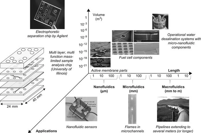
Figure 1.1 A conceptual figure which shows the common length scales spanned by microfluidics and nanofluidics along with a few examples of devices and systems. The macroscale pipeline is used as an example to provide a reference.

An identifying feature of all μ-Nafl systems is the surface-area-to-volume (SA/V) ratio. Consider two examples: (1) a simple circular cross-section nanopipe with a diameter of 10 nm and a length of 1 μm will have a SA/V ratio on the order of 10⁷ m⁻¹ and (2) a microchannel with a rectangular cross-section with a width of 100 μm, depth of 20 μm, and a length of 1 mm will have an SA/V ratio on the order of 10⁵ m⁻¹. The discussion for SA/V ratios is pertinent because several forces and related phenomena important to fluid transport at these length scales change as SA/V ratios increase, as the governing principles dominating these phenomena assume different relative magnitudes. For example, in the nanopipe example above, if the walls of the nanopipe have an electric charge, the surface of the channel will exert an electrostatic force. Since the charge is distributed over the channel or pipe area along the walls, the areas charge density becomes an important consideration. Therefore, to set up a simple scaling law comparing any surface-area term to a volume term we see that,

(1.1)

where l_c denotes characteristic length.

Consequently,

(1.2)

Equation (1.2) implies that surface-driven terms (see Chapter 3 for more details) will dominate as volumes decrease with reducing characteristic lengths. In Figure 1.2, we illustrate the concept of various phenomena that are influenced by the SA/V ratio and can be important in designing and constructing μ-Nafl systems. In turn, this gives insight to how the equations and fundamental principles can be used for implementing the ideas to building successful devices and systems.

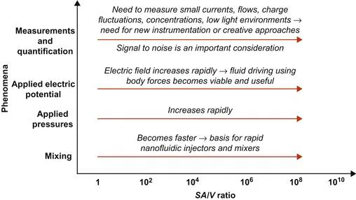
Figure 1.2 A conceptual schematic showing some of the important phenomena that influence μ-Nafl systems as function of SA/V ratios.

Following our discussion, scaling analysis can therefore provide insight to how fluid phenomena in μ-Nafl may occur in contrast to the macroscale counterparts. It should be noted that scaling analyses typically provide broad ideas and trends but more detailed experimentation and analysis may be needed for specific details. Figure 1.2 discusses several critical aspects of the scaling analysis in a brief, pictorial representation. Let us begin by considering mixing. Often in several μ-Nafl systems (see examples in Chapters 5 and 6), there is a need to bring in distinct fluid streams and allow these to mix. Due to confinement of the fluid in a device with large SA/V ratios, often the viscous and surface effects will dominate the flow phenomena (see Chapter 3 for further details), and consequently, mixing is largely driven by molecular diffusion. The time scales for molecular diffusion can be expressed as

(1.3)

where t_d is the diffusion time scale, l_c is the characteristic length, and D_AB is the diffusion coefficient of the species of interest. Equation (1.3) shows the diffusion time scales as the square of the characteristic length. Consequently, as we approach the nanoscale with decreasing l_c, time scales needed for diffusion decrease rapidly. For example, if we compare two devices and, one device has half that of the other, the smallest l_c device needs four times less time to mix the same species by diffusion as compared to the device with larger l_c. This scaling has permitted development of rapid mixers and injectors for nanoscale mixing and schemes for generating vortex-like structures at the interface of micro- and nanochannels to enhance mixing.

As we discuss in detail in Chapter 2, μ-Nafl systems with aqueous electrolyte solutions usually operate using principles of electrokinetics or using an applied electric potential to generate a body force that drives the fluid flow as opposed to pressure commonly used at the macroscale. Therefore, let us consider the scaling of a force due to the electric field. From electrostatics, the force F on a charge (let us say an ion or particle in the flow field; see Figure 1.3.) q in an electric field E is given by,

(1.4)

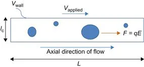
Figure 1.3 A schematic depicting a channel with flow and the forces due to an electric field shown in the axial direction. Note that the potential at the wall due to a finite wall surface density, σ_s, will also cause a force on any particles in the fluid. A more detailed discussion of the forces and the consequences in terms of flow phenomena and formation of electric double layers are discussed in Chapters 2 and 3.

For a simple scaling analysis here, we will consider a 1-D field and look at the magnitudes, so we will not consider the directionality or the vector nature of the forces in this discussion. The electric field is usually scaled as a function of the length, L across the potential drop; therefore, for an applied potential V the electric field is given by,

(1.5)

It can be noted from Eq. (1.5) that the electric fie...

Table of contents

• Cover image
• Title page
• Table of Contents
• Copyright
• Preface
• About the Authors
• Acknowledgments
• Nomenclature List
• Chapter 1. Introduction
• Chapter 2. Fundamentals for Microscale and Nanoscale Flows
• Chapter 3. Interfaces in Microfluidic and Nanofluidic Systems
• Chapter 4. Advanced Fabrication Methods and Techniques
• Chapter 5. Lab-on-a-Chip and Fluid Manipulation Applications
• Chapter 6. Energy and Environmental Applications
• A. Review of Mathematical Concepts
• Appendix B. Useful Tabulated Data
• Index