Bacterial Growth and Division

Biochemistry and Regulation of Prokaryotic and Eukaryotic Division Cycles

Stephen Cooper

• Publisher: Academic Press
• Year: 2012
• ISBN:
  9780080917474
• Topic: Biological Sciences
• Subtopic: Cell Biology
• Index: Biological Sciences

How does a bacterial cell grow during the division cycle? This question is answered by the codeveloper of the Cooper-Helmstetter model of DNA replication. In a unique analysis of the bacterial division cycle, Cooper considers the major cell categories (cytoplasm, DNA, and cell surface) and presents a lucid description of bacterial growth during the division cycle.

The concepts of bacterial physiology from Ole Maaløe's Copenhagen school are presented throughout the book and are applied to such topics as the origin of variability, the pattern of DNA segregation, and the principles underlying growth transitions.

The results of research on E. coli are used to explain the division cycles of Caulobacter, Bacilli, Streptococci, and eukaryotes. Insightful reanalysis highlights significant similarities between these cells and E.coli.

With over 25 years of experience in the study of the bacterial division cycle, Cooper has synthesized his ideas and research into an exciting presentation. He manages to write a comprehensive volume that will be of great interest to microbiologists, cell physiologists, cell and molecular biologists, researchers in cell-cycle studies, and mathematicians and engineering scientists interested in modeling cell growth.

• Written by one of the codiscoverers of the Cooper-Helmstetter model
• Applies the results of research on E. coli to other groups, including Caulobacter, Bacilli, Streptococci, and eukaryotes; the Caulobacter reanalysis highlights significant similarities with the E. coli system
• Presents a unified description of the bacterial division cycle with relevance to eukaryotic systems
• Addresses the concepts of the Copenhagen School in a new and original way

1

Bacterial Growth

I. THE STUDY OF BACTERIAL GROWTH

Bacteria grow in different ecological niches and have varied patterns of growth. This book proposes that a single, archetypal description of the pattern and regulation of cell growth and division can accommodate these myriad patterns. In order to present and apply such a model, we must first have a system that can be fully described. The defined system we shall adopt is the growth of bacteria in a laboratory culture. Many call growth in the laboratory artificial and unrepresentative; they argue that most bacteria growing in nature are starving, and usually adhering to surfaces. Exponential growth in the laboratory with unlimited medium is therefore unrepresentative. The answer to this criticism is that cell growth under laboratory conditions is analyzable and reproducible. Further, the natural situation can be explained by ideas generated by laboratory growth, but the reverse is more difficult and less common.

A. Exponential Growth

When a bacterial culture growing in unlimited medium is kept below a given concentration by dilution at suitable intervals, the culture grows continuously and exponentially. If we plot the number of cells per volume (or any other property per volume) against time, a straight line is produced on semilogarithmic paper. The growth curve is specified by:

N_t = N₀·2^t/τ

where N₀ is the cell number at zero time, N_t the cell number at any time t, and τ is the doubling time of the culture. The cell number doubles every τ minutes. The line for any other cell property increases with the same doubling time as cell number; therefore, the plotted lines are parallel (Fig. 1-1). The average properties of the culture are constant with time. The extensive properties of the culture—the amount and the number— increase. The intensive properties—the average cell size, the RNA per cell, the DNA per cell, and so forth—remain constant and invariant with time. In practice, a culture can be kept growing exponentially for many hours to ensure that it is in a constant state of exponential growth. It is not unusual to have cells growing exponentially for up to 15 hours before performing an experiment.

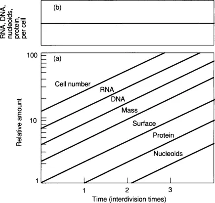
Figure 1.1 Balanced Growth of a Bacterial Culture. Determinations of the cell number, DNA, RNA, protein, or any property of cells in balanced growth give straight, parallel lines when plotted on semilogarithmic graph paper [panel (a)]. As the rates of increase of all cell properties are the same at all times, the average cell composition is constant. This is plotted in the upper graph where the cell composition is constant [panel (b)].

B. Balanced Growth

Such an exponentially growing culture can be said to be in balanced growth.¹ In most textbooks on bacteriology, the growth of bacteria is usually presented as a curve in which an overgrown culture is inoculated into fresh medium. There is lag phase before cell number begins to increase, and then a period of time when the number increases, referred to as early-, middle-, and late-log² phases. The culture stops growing as it enters stationary phase, and a final death phase may follow. This growth pattern is not an example of balanced growth. Balanced growth occurs only in that middle phase of the classic growth cycle in which cells are growing exponentially with constant properties. One of the benefits of considering balanced growth is that cultures in balanced growth have constant properties. One need not consider the problem of obtaining a reproducible physiological state for each experiment. In balanced exponential growth, the properties of the cells are ahistorical. The cell properties are independent of the age of the culture. Any results obtained are independent of the precise time when samples were removed from a culture.

The lesson of this discussion should not be missed. The terms early-log, mid-log, and late-log phase are phrases that should be eliminated from the scientific literature. Such terms may be satisfactory merely to describe harvested cells irrespective of their physiological state. In experiments where the physiological state of the bacteria is important, however, such terms are ill-defined and irreproducible. Physiological experiments should use cells in balanced growth. Experiments in which the precise physiology of the cells is unimportant could describe the precise optical density or cell density when cells were harvested or analyzed; their position in the life cycle would be unimportant; growing cells for enzyme production would be one example. Only by being careful with the growth of bacteria will the concept of log, or balanced, growth be made a rigorous and useful concept.

C. The Age Distribution

Consider a bacterial culture in which all cells are growing with precisely the same interdivision time; there is no variability in the interdivision times. The doubling time, τ, of a culture is obtained by measuring the time required for any of the properties in Fig. 1-1 to double. The time for this culture to double is the same as the time between cell divisions. A newborn cell, usually referred to as a daughter or baby cell, originates by division of a mother cell. A baby cell has an age of 0.0 and a mother cell, an age of 1.0. Cells of intermediate age are referred to by their fractional age with a cell halfway between birth and division having an age of 0.5.

What is the age distribution of an exponentially growing culture? How many cells of each age are found in an exponentially growing culture? The age distribution is a plot of the cell frequency as a function of age. We might initially think that the age distribution of a growing culture is random or uniform. There are, however, twice as many newborn cells (age 0.0) as dividing cells (age 1.0), and there is a smooth distribution of cells between these ages. The age distribution is described by:³

F_α = 2^(1−α)

where F_α is the fraction of cells at age α during the division cycle.

The ideal age distribution is plotted in Fig. 1-2. At age zero the relative frequency is 2.0, at age 1.0 the relative frequency is 1.0, and at age 0.5 the relative frequency is 1.41. A simple proof of this distribution is illustrated in Fig. 1-3 where growth is plotted on a semilogarithmic graph. At time zero, there is a population of cells that will divide within the next doubling time. Consider the cell number increase during a short interval δt₁ at the start of the plot. This time interval is associated with a cell number increase δn₁. In the last time interval, δt₂, there is a cell increase δn₂. Inspection of semilogarithmic graph paper indicates that the increase in cell number at the end of the doubling time is approximately twice that at the start of growth. At the limit (δt→0), δn₂=2·δn₁. The cell increase at the beginning of the doubling time is due to the existing cells that are just about to divide in the original culture at time zero, and the cell increase at the end of the doubling time is due to the existing cells that were just born in the culture, since these newborn cells must wait for one doubling time before they again divide. It follows that there must have been twice as many newborn cells as mother cells in the original culture at time zero. As the properties of a culture in balanced growth do not change with time, during balanced exponential growth the number of newborn cells is twice that of the mother cells.

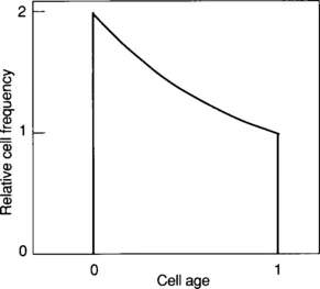
Figure 1.2 Age Distribution during Balanced Growth. The relative frequency of cells of different ages is plotted against cell age. In an ideal culture, where all interdivision times are equal, there are exactly twice as many young cells as old cells.

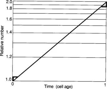
Figure 1.3 Graphic Proof of the Age Distribution. The growth of a cell culture is plotted over one interdivision time. At the left and right of the graph the rise in cell number for a short time is shown. The absolute vertical increase for the two triangles is different, with the increase at the end of the growth period twice as large as that at the start of the growth period. This is owing to the logarithmic scale. The increase at the end of the growth period is due to the existing younger or newborn cells in the culture at time zero, and the increase at the start of the growth period is due to the oldest cells that were just about to divide, so it can be seen that there must have been twice as many young cells as old cells at time zero.

The age distribution is time-invariant, and therefore the age of the average cell is constant through time. As a simple demonstration, assume that the age distribution was chosen to be artificially uniform, with all cell ages represented equally. The average age of the cells would be 0.5. An instant later each of the cells would move up from one age interval to the next. For all cells except the youngest cells, the number of cells in the interval would remain the same. The oldest cells divide to yield two young cells, so the number of cells in the youngest interval would be twice the num...

Table of contents

• Cover image
• Title page
• Table of Contents
• Dedication
• Copyright
• Acknowledgments
• Illustrations
• Tables
• Prologue
• Chapter 1: Bacterial Growth
• Chapter 2: A General Model of the Bacterial Division Cycle
• Chapter 3: Experimental Analysis of the Bacterial Division Cycle
• Chapter 4: Cytoplasm Synthesis during the Division Cycle
• Chapter 5: DNA Replication during the Bacterial Division Cycle
• Chapter 6: Synthesis of the Cell Surface during the Division Cycle
• Chapter 7: Density and Turgor during the Division Cycle
• Chapter 8: Variability of the Division Cycle
• Chapter 9: The Segregation of DNA and the Cell Surface
• Chapter 10: Transitions and the Bacterial Life Cycle
• Chapter 11: The Division Cycle of Caulobacter crescentus
• Chapter 12: Growth and Division of Streptococcus
• Chapter 13: Growth and Division of Bacillus
• Chapter 14: The Growth Law and Other Topics
• Chapter 15: The Eukaryotic Division Cycle
• Chapter 16: Conservation Laws of the Division Cycle
• Epilogue
• Bibliography
• Author Index
• Subject Index