Digital Audio Theory

A Practical Guide

Christopher L. Bennett

• Publisher: Focal Press
• Year: 2020
• ISBN:
  9781000292299
• Edition: 1
• Topic: Computer Science
• Subtopic: Digital Media
• Index: Computer Science

Digital Audio Theory: A Practical Guide bridges the fundamental concepts and equations of digital audio with their real-world implementation in an accessible introduction, with dozens of programming examples and projects.

Starting with digital audio conversion, then segueing into filtering, and finally real-time spectral processing, Digital Audio Theory introduces the uninitiated reader to signal processing principles and techniques used in audio effects and virtual instruments that are found in digital audio workstations. Every chapter includes programming snippets for the reader to hear, explore, and experiment with digital audio concepts. Practical projects challenge the reader, providing hands-on experience in designing real-time audio effects, building FIR and IIR filters, applying noise reduction and feedback control, measuring impulse responses, software synthesis, and much more.

Music technologists, recording engineers, and students of these fields will welcome Bennett's approach, which targets readers with a background in music, sound, and recording. This guide is suitable for all levels of knowledge in mathematics, signals and systems, and linear circuits. Code for the programming examples and accompanying videos made by the author can be found on the companion website, DigitalAudioTheory.com.

1

Introduction

• 1.1 Describing audio signals
• 1.2 Digital audio basics
• 1.3 Describing audio systems
• 1.4 Further reading
• 1.5 Challenges
• 1.6 Project – audio playback

If you’ve had prior experience with a Digital Audio Workstation (DAW), then you already have some idea of how audio flows from the sound source, such as a microphone or synthesizer into the DAW via an audio interface for processing, then back out for reproduction over loudspeaker or headphones. This encompasses the capture of analog audio and its conversion to digital audio, the processing of digital audio with filters and effects, and finally the conversion of digital audio for reproduction as analog sound. In Digital Audio Theory, the theoretical underpinnings of this signal chain will be examined, with an emphasis on practically implementing the theory in a signal processing environment such as Matlab® or Octave.

The digital audio signal flow to capture, process, and reproduce audio begins and ends with the converters; namely, the analog to digital converter (ADC) and the digital to analog converter (DAC). These converters are an interface between digital audio and analog representation of audio, normally voltage. Within the digital domain, typical operations of digital audio often include storage to disk, processing with a digital effect, or analysis of frequency content. The mathematical framework and practical implementation of this process will be the purview of Digital Audio Theory (Figure 1.1).

Figure 1.1
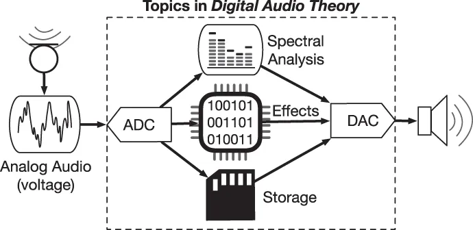
Overview of topics covered in this text, which include analog/digital conversion, linear effects (such as filters), spectral analysis, and processing.

1.1 Describing audio signals

When recording analog sound, it is useful to classify the captured audio as either desired or undesired (let’s call the latter “noise”). This classification depends on the type of sound we hope to capture – typically we might think of an instrumentalist, vocalist, or speech signal, but the numbers of categories are nearly endless, they could be ecological (e.g., urban soundscape or wildlife sounds), physiological (e.g., lung or cardiovascular sounds), among many others. However, what could be considered our desired signal in one context, could be considered noise in another. For example, environmental sounds at a sporting event are often intentionally mixed in with the broadcast to give a sense of immersion, but these same environmental sounds may be considered noise when capturing film dialog. In addition to the ambient soundscape captured by a microphone, we could also add other types of noise, including electrical (e.g., ground hum or hiss) and mechanical (e.g., vibrations of the microphone). Each of these can further be classified by their duration; transient sounds are short duration while steady-state sounds ongoing or periodic.

1.1.1 Measuring audio levels

With acoustic sound, we measure its level in units of pressure, the Pascal (Pa), which is simply force over an area (N/m²). When sound travels through air, we are not measuring the actual pressure of the air, but rather the pressure fluctuation around static pressure, which is around 101,325 Pa at sea level. Sound Pressure Level (SPL) fluctuations about static pressure that would typically be captured range anywhere from less than 1 mPa to as great as 10 Pa. The level of an acoustic audio signal can be reported as its absolute peak amplitude (known as peak SPL), or the range from its lowest trough to its highest peak (peak-to-peak SPL), or as its average value, typically reported as its root-mean-square (RMS) value. Unless otherwise specified, an SPL value can be assumed to be the RMS level, given by:

$\begin{array}{c}{x}_{RMS}=\sqrt{\frac{1}{N}{\displaystyle \sum }_{n=1}^N{x}_n^2}\end{array}(1.1)$

This equation tells us to take every value in our audio signal, x_n, and square it. Then sum all of those values together and divide by the total number of values, N, giving the average of the squared values. Finally, we take the square root of the mean of the squared values to obtain the RMS.

Without diving into psychoacoustics, or the study of the perception of sound, it can be noted that our ears perceive sound logarithmically. This applies to both SPL as well as frequency. For example, a doubling of frequency corresponds to an octave jump. To the human ear, an octave interval sounds the same, irrespective of the starting frequency. For example, the interval from 100 Hz to 200 Hz (a 100 Hz range) sounds perceptually similar to the interval from 200 Hz to 400 Hz (a 200 Hz range). For this reason, the ear is said to hear frequencies on a logarithmic base-2 scale, or log₂. For SPLs, the ear also hears logarithmically, but we use base-10 instead, or log₁₀. The unit that audio is typically reported in is a decibel (dB_SPL), defined as

$\begin{array}{c}d{\text{B}}_{\text{SPL}}\left(x_{RMS}\right)=20\cdot {\log }_{10}\left(\frac{x_{RMS}}{20\mu \text{Pa}}\right)\end{array}(1.2)$

Here, the signal, x_RMS, is converted to a logarithmic scale, with a reference of 20 μPa, the quietest SPL perceivable by the human ear. It is not uncommon to see dB_SPL reported simply as “dB”, but this is incorrect since a dB is strictly a ratio between any two values, while a dB_SPL is a ratio between a SPL and 20 μPa. Another common dB unit in audio is dB_Full-Scale, or simple dB_FS. “Full Scale” refers to the dB ratio between an audio level and the maximum representable level by the system, therefore the unit dB_FS could be thought of as the dB below Full Scale. In a digital audio system, the largest representable value is fixed – we can assign this level any arbitrary value, but 1.0 is typical. If we measure, in the same digital audio system, a signal with an RMS level of 0.1, then its dB_FS can be calculated as

$\begin{array}{c}d{\text{B}}_{\text{FS}}\left(0.1\right)=20\cdot {\log }_{10}\left(\frac{0.1}{1.0}\right)=-20{\text{dB}}_{\text{FS}}\end{array}(1.3)$

1.1.2 Pro-audio versus Consumer audio levels

You may also be familiar with the units dBu and dBv. Just like with dB_SPL, the letters “u” and “v” indicate a specific reference value. The reference for dBv is 1 Volt (V) – this is the reference that is used for consumer audio. The consumer audio standard level, which is −10 dBv, corresponds to an RMS voltage level of ${10}^{\frac{-10}{20}}\cdot 1.0=0.316\text{V}$. On the other hand, pro audio, which is reported in dBu, uses a reference voltage of 0.775 V. This voltage represents the level at which 1 milliWatt (mW) of power is achieved across a 600 Ohm (Ω) load, which was a historical standard impedance for audio e...

Table of contents

• Cover
• Half Title
• Title Page
• Copyright Page
• Dedication
• Table of Contents
• List of abbreviations
• List of variables
• 1 Introduction
• 2 Complex vectors and phasors
• 3 Sampling
• 4 Aliasing and reconstruction
• 5 Quantization
• 6 Dither
• 7 DSP basics
• 8 FIR filters
• 9 z-Domain
• 10 IIR filters
• 11 Impulse response measurements
• 12 Discrete Fourier transform
• 13 Real-time spectral processing
• 14 Analog modeling
• Index