Applying Regression and Correlation

A Guide for Students and Researchers

Jeremy Miles, Mark Shevlin

• Publisher: SAGE Publications Ltd
• Year: 2000
• ISBN:
  9781446232897
• Edition: 1
• Topic: Social Sciences
• Subtopic: Social Science Research & Methodology
• Index: Social Sciences

This book takes a fresh look at applying regression analysis in the behavioural sciences by introducing the reader to regression analysis through a simple model-building approach.

The authors start with the basics and begin by re-visiting the mean, and the standard deviation, with which most readers will already be familiar, and show that they can be thought of a least squares model. The book then shows that this least squares model is actually a special case of a regression analysis and can be extended to deal with first one, and then more than one independent variable.

Extending the model from the mean to a regression analysis provides a powerful, but simple, way of thinking about what students believe are the more complex aspects of regression analysis.

The authors gradually extend the model to include aspects of regression analysis such as non-linear regression, logistic regression, and moderator and mediator analysis. These approaches are often presented in terms that are too mathematical for non-statistically inclined students to deal with.

Throughout the book maintains a conceptual, non-mathematical focus. Most equations are placed in an appendix, where a detailed explanation is given, to avoid disrupting the flow of the main text.

This book will be indispensable for anyone using regression and correlation from undergraduates doing projects to postgraduate and researchers.

PART I

I NEED TO DO REGRESSION ANALYSIS TOMORROW

1 Building models with regression and correlation

1.1 What are models?

How tall do you (the reader) think we (the authors) are? Decide your answer before you read on.

Your answer may have been, ‘What a stupid question’ or ‘How should I know?’ If you think about it, the question is not very stupid, and you should have some idea. You can see (from our names on the front cover) that we are both male. You can safely assume that we are not so young that we are not fully grown, and we will tell you that we did not start smoking until we had almost reached our full adult heights, thus stunting our growth only a little. Given this, you know that we are not 4 inches tall, nor are we 100 feet tall. A reasonable guess, given the information that you have, would be that we are of about average height for males – approximately 5 feet and 10 inches (1.77 m). We are in fact both slightly over 6 feet (1.83 m) tall, so if you had guessed the average height, your guess would have been a couple of inches out – not bad really.

What you did was to build a model. Your model was ‘The authors are 5 feet 10 inches tall.’ This is a model of our heights – it is a very simple model, but a model nonetheless. A model is a representation of the world, but it is rarely a perfect representation. There will always be some differences between the model and the world, that is some error. If we could build a perfect copy, it would not be a model, it would be a duplicate.

What you did when trying to guess our height was to pick a value that had as little error in it as possible. The value with the least chance of error would be the average height. There is more chance of us being average than being unusual – that’s what averages are. Your model was as close as possible to the data (our heights), but there was some error remaining. A different way of saying this is that:

DATA = MODEL + ERROR

This is a very important statement, which we shall refer to a lot throughout this chapter, so let’s look at a practical example.

Imagine that we have some data on the number of books on research methods and statistics that a small group of psychology students has read during their studies. Table 1.1 shows these data.

TABLE 1.1

Name	Number of books read
Anne	2
Bob	4
Carol	1
David	0
Esther	3

If we want to model those data, we could do it by repeating the numbers. We could say 2, 4, 1, 0, 3. The numbers that make up the model are known as parameters, and this model has five of them.

In terms of:

DATA = MODEL + ERROR

DATA are equal to MODEL, and so ERROR is zero; there is no difference between the model and the data. This model is a perfect representation of the data. However, there is a problem with this model. There were five numbers in the data, and there are five numbers (or parameters) in the model, so the model has not summarised anything – it is not really a model, but a duplicate. A model should be a simple, or parsimonious, representation of a phenomenon. In this case the model is the data, and we are back where we started (so in fact we could argue that this is not a model at all). That the model and the data are exactly the same is not much of a problem when we are dealing with five numbers, but if we are trying to summarise 500 numbers, this approach will not work, so we need a different approach.

If we want to model the data with one parameter, we could use the mean. This is what people commonly call the average (although it is better to avoid this term as it has more than one definition). To find the mean score, we add together the five numbers (sum the set of numbers), and divide this sum or total by the number of people:

2 + 4 + 1 + 0 + 3 = 10
10/5 = 2

We have calculated that the mean number of books on statistics read by these psychology students is two.¹ We have used the mean as a simple model, which has one parameter, and describes the data.

1.2 Least squares models

1.2.1 A very simple model

We saw in the previous section that we used a model that contained one parameter, the mean, to represent a set of five numbers. We used the mean for a good reason because it summarised the data: with just one number, it gives us a general idea about a whole set of numbers.

The mean is a special type of model; it is a least squares model. In this section, we shall see what we mean by a least squares model, and find out why the fact that the mean is a least squares model is important. Remember that (we said we would keep coming back to this):

DATA = MODEL + ERROR

DATA was the number of books read by each student; the numbers 2, 4, 1, 0, 3. Our model is the mean, the number 2. The difference between the model and the data is ERROR. If:

DATA = MODEL + ERROR

it is also true that:

ERROR = DATA – MODEL

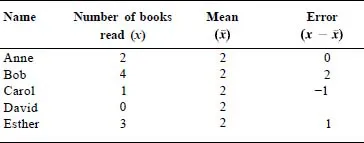
Table 1.2 shows the number of books that each student has read along with the differences between the number for each student and the model (the mean). The difference between the model and the number of books read by a particular student is what we call the error for that student.

TABLE 1.2

In statistics, the errors (or differences) such as those shown in the table are sometimes called residuals. The residuals are what are left over after the model (mean) has been taken away from each student’s score. They are the difference between the score predicted by the model and the score that each individual actually has.

We said earlier that the model we were going to select was the model that gave the least error. We picked the mean height for males as your model for the heights of the authors of this book because that would have been your best guess. The score for each person is the mean plus (or minus) some error.

Often in statistics, we want to refer to a whole set of numbers, rather than just one individual number. For example, where we have a set of numbers that refer to the number of books read, we would call this x. We will often call this a variable, as it is something that can vary between people. You may also see it referred to as a ‘vector’ in more mathematically inclined texts. We can refer to the first number in the variables (or vector) as x₁, the second as x₂, etc. We can write Table 1.2 as:

The above list is the statistical way of saying that the score for the first person is equal to the mean plus the residual for the first person, the score for the second person is equal to the mean plus the residual for the second person, and so on. In statistics, we can use the subscript i for the individuals. Instead of writing out the full set of equations, as we did above, we can write:

This means ‘take this equation and repeat it for every person’. Sometimes statisticia...

Table of contents

• Cover Page
• Title
• Copyright
• Contents
• Preface
• Part I: I need to do Regression Analysis Tomorrow
• Part II: I need to do Regression Analysis Next Week
• Part III: I need to know more of The Things that Regression Can do
• Appendix 1 Equations
• Appendix 2 Doing regression with SPSS
• Appendix 3 Statistical tables
• References
• Name index
• Subject index