Applied Regression and Modeling

Amar Sahay

• Publisher: Business Expert Press
• Year: 2016
• ISBN:
  9781631573309
• Topic: Business
• Subtopic: Operations
• Index: Business

The book is divided into three parts – (1) prerequisite to regression analysis followed by a discussion on simple regression, (2) multiple regression analysis with applications, and (3) regression and modeling including the second order models, nonlinear regression, and interaction models in regressions. All these sections provide examples with complete computer analysis and instructions commonly used in modeling and analyzing these problems. The book deals with detailed analysis and interpretation of computer results. This will help readers to appreciate the power of computer in applying regression models. The readers will find that the understanding of computer results is critical to implementing regression and modeling in real world situation. The book is written for juniors, seniors and graduate students in business, MBAs, professional MBAs, and working people in business and industry. Managers, practitioners, professionals, quality professionals, quality engineers, and anyone involved in data analysis, business analytics, and quality and six sigma will find the book to be a valuable resource.

CHAPTER 1

Introduction to Regression and Correlation Analysis

Introduction

In real world, managers are always faced with massive amount of data involving several different variables. For example, they may have data on sales, advertising, or the demand for one of the several products his or her company markets. The data on each of these categories—sales, advertising, and demand is a variable. Any time we collect data on any entity, we call it a variable and statistics is used to study the variation in the data. Using statistical tools we can also extract relationships between different variables of interest. In dealing with different variables, often a question arises regarding the relationship between the variables being studied. In order to make effective decisions, it is important to know and understand how the variables in question are related. Sometimes, when faced with data having numerous variables, the decision-making process is even more complicated. The objective of this text is to explore the tools that will help the managers investigate the relationship between different variables. The relationships are critical to making effective decisions. They also help to predict one variable using the other variable or variables of interest.

The relationship between two or more variables is investigated using one of the most widely used tools—regression and correlation analysis. Regression analysis is used to study and explain the mathematical relationship between two or more variables. By mathematical relationship we mean whether the relationship between the variables is linear or nonlinear. Sometimes we may be interested in only two variables. For example, we may be interested in the relationship between sales and advertising. Companies spend millions of dollars in advertising and expect that an increase in the advertising expenditure will significantly improve the sales. Thus, these two variables are related. Other examples where two variables might be related are production cost and the volume of production, increase in summer temperature and the cooling cost, or the size of house in square-feet and its price. Once the relationship between two variables is explained, we can predict one of the variables using the other variable. For example, if we can establish a strong relationship between sales and advertising, we can predict the sales using advertising expenditure. This can be done using a mathematical relationship (to be explained later) between sales and advertising. There is another tool often used in conjunction with regression analysis known as correlation analysis. This correlation explains the degree of association between the two variables; that is, it explains how strong or weak the relationship between the two variables is.

The relationship between two variables is explained and studied using the technique of simple regression analysis. Managers are also faced with situations where many variables are involved. In such cases, they might be interested in the possible relationship between these variables. They may also be interested in predicting one variable using several variables. This problem is more involved and complex due to multiple variables involved. The problem involving many variables is studied using the technique of multiple regression analysis. Owing to the complex nature of multiple regression problems, computers are almost always used for this analysis.

The objective in simple regression is to predict one variable using the other. The variable to be predicted is known as the dependent or response variable and the other one is known as the independent variable or predictor. Thus, the problem of simple regression involves one dependent and one independent variable. An example would be to predict the sales (the dependent variable) using the advertising expenditure (the independent variable). In multiple regression problems, where the relationship between multiple variables is of interest, the objective is to predict one variable—the dependent variable using the other variables known as independent variables. An example of multiple regression would be to predict the sales for a grocery chain using the food-item sales, nonfood-item sales, size of the store, and the operating hours (12 or 24 hours). The multiple regression problem involves one dependent and two or more independent variables.

The problems of simple and multiple linear regressions assume that the relationship between the variables is linear. This is the reason these are referred to as the simple linear regression and multiple linear regression. It is important to note that the relationship between the variables is not always linear. Sometimes, a linear relationship between the variables may not exist. In such cases, the relationship between the variables can be best explained using a nonlinear relationship. By nonlinear relationships, we mean a curvilinear relationship that can be described using a quadratic or second-order or higher order equation. In analyzing such complex regression models, a computer package is almost always used. In this text, we have used Excel and MINITAB^® computer packages to analyze the regression models. We have demonstrated the applications of simple, multiple, and higher order regressions using these software. The reason for using Excel is obvious. It is one of the most widely used spreadsheet programs in industry and academia. MINITAB is the leading statistical software for quality improvement and is used by 90% of Fortune 100 companies. It is also widely used as a teaching tool in colleges and universities. It is worth mentioning at this point that Excel is a spreadsheet program and was not designed for performing in-depth statistical analysis. It can be used for analyses up to a certain level but lacks the capability of producing in-depth reports for higher order regression models. If you perform regression analysis with substantial amount of data and need more detailed analyses, the use of statistical package such as MINITAB, SSS^®, and SPSS^® is recommended.

The statistical concepts needed for regression are included in Appendix B. This includes a review of statistical techniques that are necessary in explaining and building regression models. The graphical and numerical methods used in statistics and some more background information including the sampling, estimation and confidence intervals, and hypothesis testing are provided in Appendix B. The readers can download the Appendix at their convenience through a link provided. In the subsequent chapters of the book, we discuss and provide complete analysis (including computer analysis) and interpretation of simple and multiple regression analysis with applications; regression and modeling including second-order models, nonlinear regression, regression models using qualitative (dummy) variables, and interaction models. All these sections provide examples with complete computer analysis and interpretation of regression and modeling using real-world data and examples. The detailed analysis and interpretation of computer results using widely used software packages will help readers to gain an understanding of regression models and appreciate the power of computer in solving such problems. All the data files in both MINITAB and Excel formats are provided in separate folders. The step-wise computer instructions are provided in Appendix A of the book. The readers will find that the understanding of computer results is critical to implementing regression and modeling in real-world situations.

Before we describe the regression models and the statistical and mathematical basis behind them, we present some fundamental concepts and graphical techniques that are helpful in studying the relationships between the variables.

Measures of Association Between Two Quantitative Variables: The Scatterplot and the Coefficient of Correlation

Describing the relationship between two quantitative variables is called a bivariate relationship. One way of investigating this relationship is to construct a scatterplot. A scatterplot is a two-dimensional plot where one variable is plotted along the vertical axis and the other along the horizontal axis. The pairs of points (x_i, y_i) plotted on the scatterplot are helpful in visually examining the relationship between the two variables.

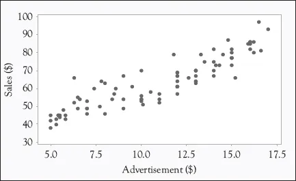
In a scatterplot, one of the variables is considered a dependent variable and the other an independent variable. The data value is thought of as having a (x, y) pair. Thus, we have (x_i, y_i), i = 1, 2, ..., n pairs. One of the easiest ways to explain the relationship between the two variables is to plot the (x, y) pairs in the form of a scatterplot. Computer packages such as Excel and MINITAB provide several options for constructing scatterplots. Figure 1.1 shows a scatterplot depicting the relationship between sales and advertising expenditure for a company (Data file: SALES&AD.MTW).

From Figure 1.1, we can see a distinct increase in sales associated with the higher values of advertisement dollars. This is an indication of a positive relationship between the two variables where we can see a positive trend. This means that an increase in one variable leads to an increase in the other.

Figure 1.1 Scatterplot of sales versus advertisement

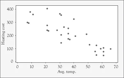
Figure 1.2 A scatterplot depicting inverse relationship between heating cost and temperature

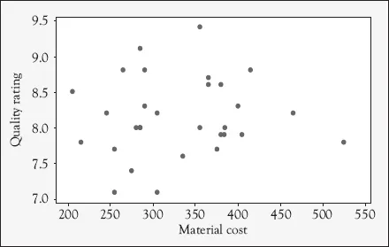
Figure 1.2 shows the relationship between the home heating cost and the average outside temperature (Data File: HEAT.MTW). This plot shows a tendency for the points to follow a straight line with a negative slope. This means that there is an inverse or negative relationship between the heating cost and the average temperature. As the average outside temperature increases, the home heating cost goes down. Figure 1.3 shows a weak or no relationship between quality rating and material cost of a product (Data File RATING.MTW).

Figure 1.3 Scatterplot of quality rating and material cost (weak or no relationship)

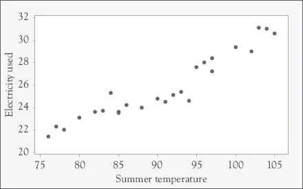
Figure 1.4 A scatterplot of summer temperature and electricity used

In Figure 1.4, we have plotted the summer temperature and the amount of electricity used (in millions of kilowatts) (Data File: SCATTER1.MTW). The plotted points in this figure can be well approximated by a straight line. Therefore, we can conclude that a linear relationship exists between the two variables.

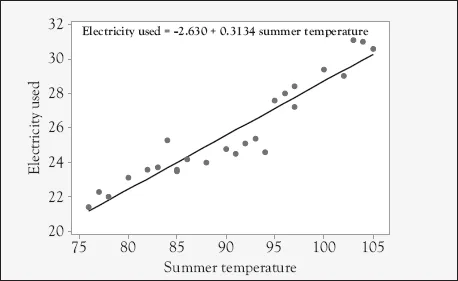
The linear relationship can be explained by plotting a regression line over the scatterplot as shown in Figure 1.5. The equation of this line is used to describe the relationship between the two variables—temperature and electricity used.

Figure 1.5 Scatterplot with regression line

These plots demonstrate the relationship between two variables visually. The plots are very helpful in explaining the types of relationship between the two variables and are usually the first step in studying such relationships. The regression line shown in Figure 1.5 is known as the line of “best fit.” This is the best-fitting line through the data points and is uniquely determined using a mathematical technique known as the least squares method. We will explain the least squares method in detail in the subsequent chapters. In regression, the least squares method is used to determine the best-fitting line or curve through the data po...

Table of contents

• Cover
• Title
• Copyright
• Preface
• Acknowledgments
• Computer Software Integration, Computer Instructions, and Data Files
• Chapter 1. Introduction to Regression and Correlation Analysis
• Chapter 2. Regression, Covariance, and Coefficient of Correlation
• Chapter 3. Illustration of Least Squares Regression Method
• Chapter 4. Regression Analysis Using a Computer
• Chapter 5. Multiple Regression: Computer Analysis
• Chapter 6. Model Building and Computer Analysis
• Chapter 7. Models with Qualitative Independent (Dummy) Variables, Interaction Models, All Subset and Stepwise Regression Models with Computer Analysis
• Chapter 8. Notes on Implementation of Regression Models
• Bibliography
• Index
• Adpage