Numerical Methods for Stochastic Computations

A Spectral Method Approach

Dongbin Xiu

• Publisher: Princeton University Press
• Year: 2010
• ISBN:
  9781400835348
• Topic: Mathematics
• Subtopic: Applied Mathematics
• Index: Mathematics

The@ first graduate-level textbook to focus on fundamental aspects of numerical methods for stochastic computations, this book describes the class of numerical methods based on generalized polynomial chaos (gPC). These fast, efficient, and accurate methods are an extension of the classical spectral methods of high-dimensional random spaces. Designed to simulate complex systems subject to random inputs, these methods are widely used in many areas of computer science and engineering.
The book introduces polynomial approximation theory and probability theory; describes the basic theory of gPC methods through numerical examples and rigorous development; details the procedure for converting stochastic equations into deterministic ones; using both the Galerkin and collocation approaches; and discusses the distinct differences and challenges arising from high-dimensional problems. The last section is devoted to the application of gPC methods to critical areas such as inverse problems and data assimilation.
Ideal for use by graduate students and researchers both in the classroom and for self-study, Numerical Methods for Stochastic Computations provides the required tools for in-depth research related to stochastic computations.

• The first graduate-level textbook to focus on the fundamentals of numerical methods for stochastic computations
• Ideal introduction for graduate courses or self-study
• Fast, efficient, and accurate numerical methods
• Polynomial approximation theory and probability theory included
• Basic gPC methods illustrated through examples

Chapter One

Introduction

The goal of this chapter is to introduce the idea behind stochastic computing in the context of uncertainty quantification (UQ). Without using extensive discussions (of which there are many), we will use a simple example of a viscous Burgers’ equation to illustrate the impact of input uncertainty on the behavior of a physical system and the need to incorporate uncertainty from the beginning of the simulation and not as an afterthought.

1.1 STOCHASTIC MODELING AND UNCERTAINTY QUANTIFICATION

Scientific computing has become the main tool in many fields for understanding the physics of complex systems when experimental studies can be lengthy, expensive, inflexible, and difficulty to repeat. The ultimate goal of numerical simulations is to predict physical events or the behaviors of engineered systems. To this end, extensive efforts have been devoted to the development of efficient algorithms whose numerical errors are under control and understood. This has been the primary goal of numerical analysis, which remains an active research branch. What has been considered much less in classical numerical analysis is understanding the impact of errors, or uncertainty, in data such as parameter values and initial and boundary conditions.

The goal of UQ is to investigate the impact of such errors in data and subsequently to provide more reliable predictions for practical problems. This topic has received an increasing amount of attention in past years, especially in the context of complex systems where mathematical models can serve only as simplified and reduced representations of the true physics. Although many models have been successful in revealing quantitative connections between predictions and observations, their usage is constrained by our ability to assign accurate numerical values to various parameters in the governing equations. Uncertainty represents such variability in data and is ubiquitous because of our incomplete knowledge of the underlying physics and/or inevitable measurement errors. Hence in order to fully understand simulation results and subsequently to predict the true physics, it is imperative to incorporate uncertainty from the beginning of the simulations and not as an afterthought.

1.1.1 Burgers’ Equation: An Illustrative Example

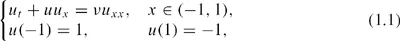
Let us consider a viscous Burgers’ equation,

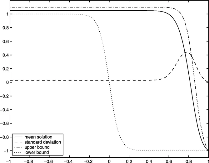
Figure 1.1 Stochastic solutions of Burgers’ equation (1.1) with u(—1, t) = 1 +δ, where δ is a uniformly distributed random variable in (0, 0.1) and v = 0.05. The solid line is the average steady-state solution, with the dotted lines denoting the bounds of the random solutions. The dashed line is the standard deviation of the solution. (Details are in [123].)

where u is the solution field and v > 0 is the viscosity. This is a well-known nonlinear partial differential equation (PDE) for which extensive results exist. The presence of viscosity smooths out the shock discontinuity that would develop otherwise. Thus, the solution has a transition layer, which is a region of rapid variation and extends over a distance of O(v) as v ↓ 0. The location of the transition layer z, defined as the zero of the solution profile u(t, z) = 0, is at zero when the solution reaches steady state. If a small amount of (positive) uncertainty exists in the value of the left boundary condition (possibly due to some bias measurement or estimation errors), i.e., u(—1) = 1+δ, where 0 < δ << 1, then the location of the transition can change significantly. For example, if δ is a uniformly distributed random variable in the range of (0, 0.1), then the average steady-state solution with v = 0.05 is the solid line in Figure 1.1. It is clear that a small uncertainty of 10 percent can cause significant changes in the final steady-state solution whose average location is approximately at z ≈ 0.8, resulting in a O(1) difference from the solution with an idealized boundary condition containing no uncertainty. (Details of the computations can be found in [123].)

The Burgers’ equation example demonstrates that for some problems, especially nonlinear ones, a small uncertainty in data may cause nonneghgible changes in the system output. Such changes cannot be captured by increasing resolution of the classical numerical algorithms if the uncertainty is not incorporated at the beginning of the computations.

1.1.2 Overview of Techniques

The importance of understanding uncertainty has been realized by many for a long time in disciplines such as civil engineering, hydrology, control, etc. Consequently many methods have been devised to tackle this issue. Because of the “uncertain” nature of the uncertainty, the most dominant approach is to treat data uncertainty as random variables or random processes and recast the original deterministic systems as stochastic systems.

We remark that these types of stochastic systems are different from classical stochastic differential equations (SDEs) where the random inputs are idealized processes such as Wiener processes, Poisson processes, etc., and tools such as stochastic calculus have been developed extensively and are still under active research. (See, for example, [36, 55, 57, 85].)

1.1.2.1 Monte Carlo- and Sampling-Based Methods

One of the most commonly used methods is Monte Carlo sampling (MCS) or one of its variants. In MCS, one generates (independent) realizations of random inputs based on their prescribed probability distribution. For each realization the data are fixed and the problem becomes deterministic. Upon solving the deterministic realizations of the problem, one collects an ensemble of solutions, i.e., realizations of the random solutions. From this ensemble, statistical information can be extracted, e.g., mean and variance. Although MCS is straightforward to apply as it only requires repetitive executions of deterministic simulations, typically a large number of executions are needed, for the solution statistics converge relatively slowly. For example, the mean value typically converges as

where K is the number of realizations (see, for example, [30]). The need for a large number of realizations for accurate results can incur an excessive computational burden, especially for systems that are already computationally intensive in their deterministic settings.

Techniques have been developed to accelerate convergence of the brute-force MCS, e.g., Latin hypercube sampling (cf. [74, 98]) and quasi Monte Carlo sampling (cf. [32, 79, 80]), to name a few. However, additional restrictions are posed based on the design of these methods, and their applicability is often limited.

1.1.2.2 Perturbation Methods

The most popular nonsampling methods were perturbation methods, where random fields are expanded via Taylor series around their mean and truncated at a certain order. Typically, at most second-order expansion is employed because the resulting system of equations becomes extremely complicated beyond the second order. This approach has been used extensively in various engineering fields [56, 71, 72]. An inherent limitation of perturbation methods is that the magnitude of the uncertainties, at both the inputs and outputs, cannot be too large (typically less than 10 percent), and the methods do not perform well otherwise.

1.1.2.3 Moment Equations

In this approach one attempts to compute the moments of the random solution directly. The unknowns are the moments of the solution, and their equations are derived by taking averages of the original stochastic governing equations. For example, the mean field is determined by the mean of the governing equations. The difficulty lies in the fact that the derivation of a moment almost always, except on some rare occasions, requires information about higher moments. This brings out the closure problem, which is often dealt with by utilizing some ad hoc arguments about the properties of the higher moments.

1.1.2.4 Operator-Based Methods

These kinds of approaches are based on manipulation of the stochastic operators in the governing equations. They include Neumann expansion, which expresses the inverse of the stochastic operator in a Neumann series [95, 131], and the weighted integral method [23, 24]. Similar to perturbation methods, these operator-based methods are also restricted to small uncertainties. Their applicability is often strongly dependent on the underlying operator and is typically limited to static problems.

1.1.2.5 Generalized Polynomial Chaos

A recently developed method, generalized polynomial chaos (gPC) [120], a generalization of classical polynomial chaos [45], has become one of the most widely used methods. With gPC, stochastic solutions are expressed as orthogonal polynomials of the input random parameters, and different types of orthogonal polynomials can be chosen to achieve better convergence. It is essentially a spectral representation in random space and exhibits fast convergence when the solution depends smoothly on the random parameters. gPC-based methods will be the focus of this book.

1.1.3 Burgers’ Equation Revisited

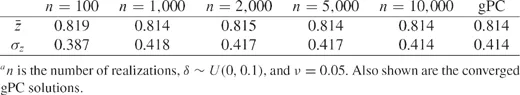
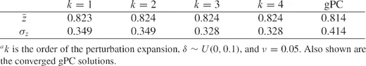
Let us return to the viscous Burgers’ example (1.1), with the same parameter settings that produced Figure 1.1. Let us examine the location of the averaged transition layer and the standard deviation of the solution at this location as obtained by different methods. Table 1.1 shows the results by Monte Carlo simulations, and Table 1.2 by a perturbation method at different orders. The converged solutions by gPC (up to three significant digits) are obtained by a fourth-order expansion and are tabulated for comparison. It can be seen that MCS achieves the same accuracy with O(10⁴) realizations. On the other hand, the computational cost of the fourth-order gPC is approximately equivalent to that for five deterministic simulations. The perturbation methods have a low computational cost similar to that of gPC. However, the accuracy of perturbation methods is much less desirable, as shown in Table 1.2. In fact, by increasing the perturbation orders, no clear convergence can be observed. This is caused by the relatively large uncertainty at the output, which can be as high as 40 percent, even though the input uncertainty is small.

Table 1.1 Mean Location of the Transition Layer

and Its Standard Deviation (σ_z) by Monte Carlo Simulations^a

Table 1.2 Mean Location of the Transition Layer

and Its Standard Deviation (σ_z) Obtained by Perturbation Methods^a

This example demonstrates the accuracy and efficiency of the gPC method. It should be remarked that although gPC shows a significant advantage here, the conclusion cannot be trivially generalized to other problems, as the strength and the weakness of gPC, or any method for that matter, are problem-dependent.

1.2 SCOPE AND AUDIENCE

As a graduate-level text, this book focuses exclusively on the fundamental aspects of gPC-based numerical methods, with a detailed exposition of their formulations, basic properties, and connections to classical numerical methods. No research topics are discussed in this book. Although this leaves out many exciting new developments in stochastic computing, it helps to keep the book self-contained, compact, and more accessible to students who want to learn the basics. The material is also chosen and organized in such a way that the book can be finished in a one-semester course. Also, the book is not intended to contain a thorough and exhaustive literature review. References are limited to those that are more accessible to graduate students.

In chapter 2, we briefly review the basic concepts of probability theory. This is followed by a brief review of approximation theory in chapter 3. The material in these two chapters is kept at almost an absolute minimum, with only the very basic concepts included. The goal of these two chapters is to prepare students for the more advanced material in the following chapters. An interesting question is how much time the instructor should dedicate to these two chapters. Students taking the course usually have some background knowledge of either numerical analysis (which gives them some preparation in approximation theory) or probability theory (or statistics), but rarely do students have both. And a comprehensive coverage of both topics can easily consume a large portion of class time and leave no time for other material. From the author’s personal teaching experience, it is better to go through probability theory rather fast, covering only the basic concepts and leaving other concepts as reading assignments. This is reflected in the writing of this book, as chapter 2 is quite concise. The approximation theory in chapter 3 deserves more time, as it is closely related to many concepts of gPC in the ensuing chapters.

In chapter 4, the procedure for formulating stochastic systems is presented, and an important step, parameterization of random inputs, is discussed in detail. A formal and systematic exposition of gPC is given in chapter 5, where some of the important properties of gPC expansion are presented. Two major numerical approaches, stochastic Galerkin and stochastic collocation, are covered in chapters 6 and 7, respectively. The algorithms are discussed in detail, along with some examples for better understanding. Again, only the basics of the algorith...

Table of contents

• Cover
• Title Page
• Copyright
• Dedication
• Contents
• Preface
• Chapter One - Introduction
• Chapter Two - Basic Concepts of Probability Theory
• Chapter Three: : Survey of Orthogonal Polynomials and Approximation Theory
• Chapter Four - Formulation of Stochastic Systems
• Chapter Five - Generalized Polynomial Chaos
• Chapter Six - Stochastic Galerkin Method
• Chapter Seven - Stochastic Collocation Method
• Chapter Eight - Miscellaneous Topics and Applications
• Appendix A - Some Important Orthogonal Polynomials in the Askey Scheme
• Appendix B - The Truncated Gaussian Model G (α, β)
• References
• Index