Introduction to Mathematical Sociology

Phillip Bonacich, Philip Lu

• Publisher: Princeton University Press
• Year: 2012
• ISBN:
  9781400842452
• Topic: Social Sciences
• Subtopic: Social Science Research & Methodology
• Index: Social Sciences

A comprehensive textbook on the tools of mathematical sociology and their applications Mathematical models and computer simulations of complex social systems have become everyday tools in sociology. Yet until now, students had no up-to-date textbook from which to learn these techniques. Introduction to Mathematical Sociology fills this gap, providing undergraduates with a comprehensive, self-contained primer on the mathematical tools and applications that sociologists use to understand social behavior.Phillip Bonacich and Philip Lu cover all the essential mathematics, including linear algebra, graph theory, set theory, game theory, and probability. They show how to apply these mathematical tools to demography; patterns of power, influence, and friendship in social networks; Markov chains; the evolution and stability of cooperation in human groups; chaotic and complex systems; and more. Introduction to Mathematical Sociology also features numerous exercises throughout, and is accompanied by easy-to-use Mathematica-based computer simulations that students can use to examine the effects of changing parameters on model behavior.

• Provides an up-to-date and self-contained introduction to mathematical sociology
• Explains essential mathematical tools and their applications
• Includes numerous exercises throughout
• Features easy-to-use computer simulations to help students master concepts

CHAPTER 1

Introduction

Mathematical sociology is not an oxymoron. There is a useful role for mathematics in the study of society and groups. In fact, that role is growing as social scientists and others develop better and better tools for the study of complex systems. A number of trends are converging to make the application of mathematics to society increasingly productive.

First, more and more human systems are complex, in a sense to be described soon. World economies are more and more interconnected. Our transportation and communication systems are increasingly worldwide. Social networks are less local and more global, making them more complex, producing new emergent communication patterns, a positive effect, but which also has made us increasingly vulnerable to pandemics, a negative effect. The Internet has connected us in ways that no one understands completely. Power grids are less and less local and are subject to more widespread failures than ever before. New species are increasingly introduced into local complex ecologies with unexpected effects. Our recent climate change has produced a situation in which it is more and more important to predict the future and the effects of human interventions in the complex system of the global weather. The mapping of the human genome makes available to biologists the possibility of studying the complex system of interactions between genes and proteins. All of these tendencies mean that scientists in a wide variety of areas—computer science, economics, ecology, genetics, climatology, epidemiology, and others—have developed mathematical tools to study complex systems, and these tools are available to us sociologists.

The second important trend is the growing power and ubiquity of the computer. Computer simulations and mathematics are complementary tools for the study of complex systems. They are two different ways of drawing implications for the future from what is known or assumed to be true. Mathematics can be used to draw far-reaching and sometimes unexpected conclusions using logic and mathematics. For example, many properties of networks have been proved to be true by mathematicians using traditional mathematical tools. Computer simulations use computer programs the coding of which embodies assumptions and whose conclusions are evident after the program has iterated. Computer simulations are useful in situations that are unsolved or intractable mathematically.

This text uses both mathematics and computer simulations. Sometimes the computer simulations demonstrate phenomena for which there is no exact mathematical solution. More frequently simulations are used to illustrate some model so that you, the reader of this book, will gain some understanding of how the model works and how it is affected by varying parameters even if a full mathematical treatment of the model is beyond the purpose of this book.

EPIDEMICS

At the time we are writing this chapter there is an epidemic of concern over swine fever, a variant of influenza that seems to have captured the public’s attention. Both the flu and fear of this flu spread through social networks, and we want now to illustrate some of the properties of epidemics through a very simple model. The model will be illustrated both with a little simple mathematics and with a computer simulation.

Suppose that a large population consists of N individuals. Suppose that each individual in the population has small probability p of being connected to each of the others in the population and that his connection to one individual has no bearing on his connection to any other person in the population. This creates a random network among the members of the population. Real social networks are not like random networks, but random networks are very tractable mathematically, and so they tend to be assumed by epidemiologists who study the spread of diseases. The powerful conclusions may be relatively unaffected by the unreality of the assumptions, much like the statistician may on occasion assume a normal distribution because the conclusions are not affected very much if the assumption of a normal distribution is not exactly true. We will examine how real social networks differ from random networks in much more detail in later chapters, but for the moment we will assume that they are useful descriptions of real networks.

Despite its unrealism, let’s, for the sake of convenience, assume that the network is random. Suppose that initially just one person is sick with a contagious disease. If p is the probability this person is connected to anyone else, then we should expect this person to be connected to p × N others, on the average. If p is small and N is large, then each of these pN individuals will be connected to pN others, and so the sick individual will be connected to (pN)² individuals indirectly, through his contacts. If p is small and N is large we can ignore the unlikely event that some individuals will be connected to more than one of his direct connections. Similarly (pN)³ persons will be connected even less directly, through two intermediaries, and (pN)^k+1 persons will be connected through k intermediaries. Let’s look at this sequence:

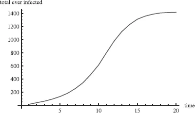
Figure 1.1. Total number of infected individuals when pN = 1.5.

This represents the expected or average number of people who get the contagious disease carried by one person. Of course, this number must in fact be limited because the population is of finite size N but if pN ≥ 1, this sum diverges: it just gets bigger and bigger, without limit. If pN < 1, however, the sum converges to a number, and this number may be quite small relative to N. The sequence in equation 1.1 converges to,

You can verify this for yourself by substituting a few values. When pN = .5, for example, the sums are 1, 1.5, 1.75, 1.875, and so on, getting closer and closer to 2, the limit. What this means is that if an infected person infects, on the average, less than one other person the disease will not become an epidemic affecting nearly everyone, but otherwise it will spread to the entire population.

The following figures were generated from a simulation based on a few simple assumptions. The network was of size 2,500. Ten individuals were initially infected. The probability that any two people were connected, also the probability that an infected person would infect a healthy person in any given time period, was set at .0006: p =.0006. The network was examined over 100 time periods. If infected in one time period, the person was assumed to be infectious at the next time period and immune thereafter. In this case p × N = .0006 × 2,500 = 1.5, and 1.5 is bigger than the critical value of 1.00 ties per person. We should expect the disease to spread.

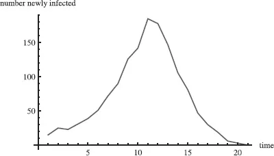
Figure 1.1 shows the total number infected. After just 25 time periods most had been infected. The curve shows a familiar S-shaped figure, called the logistic curve. The disease spread slowly when few had it, then picked up speed, then slowed down as there were fewer and fewer who had not been infected and were not immune. Figure 1.2 shows the number of new cases in each time period, telling the same story as Figure 1.1 in a different way.

Figure 1.2. Number of total and newly infected individuals over time when pN = 1.5.

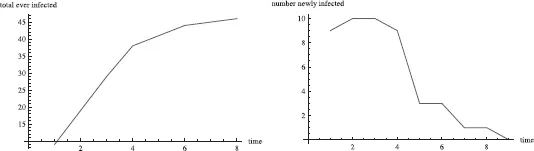
Figure 1.3. Number of newly infected individuals over time when pN = 1.5.

Now suppose we make the parameter p half as big, p = .0003, so that each individual averages .75 contacts instead of 1.50. This is below the critical value of one contact per person on average. We would expect the outbreak not to become an epidemic and to peter out after the initial set of infected individuals fail to reproduce themselves. Figure 1.3 shows that the total number never passes 50 and illustrates the declining number of new cases.

In later chapters we’ll see how these inferences are a consequence of deep and nonobvious properties of random networks. We will also see how the inferences must be modified for other classes of nonrandom networks. Even with these qualifications, the results are interesting. First, they apply to phenomena other than the spread of disease. Information and rumor transition can also be modeled. Coleman et al. (1966) used this model to account for diffusion in the use of a new antibiotic among doctors in Midwestern communities. In this case, what was being spread was not disease but information and influence. The existence of a critical point has policy implications in epidemiology. It means that not everyone need be inoculated for an inoculation campaign to be effective. It also helps explain why Apple computers are less subject to viruses than are PCs. Since computer viruses are targeted for one operating system, any Mac virus will spread only from Mac to Mac, while almost all the computers a Mac is connected to will be PCs. The Mac to Mac network will be very sparse while the PC to PC network will have a lot higher density (a higher value of p). Thus, the lower frequency of Mac infections need not be due to any superiority of the Mac operating system but simply due to the fact that very few people use Macs.

The spread of a disease or information depends not only on the density of the network but also on the presence or absence of longrange connections in the network, and this topic can be examined both mathematically and through the use of computer simulations. When in history almost all ties between people were strictly local, epidemic diseases spread much more slowly. The “Black Death,” a plague that decimated Europe in the Middle Ages, was carried by sailors from Asia to Italian port cities in 1347, but it did not reach England until 1349 and Scandinavia until 1350. This slow spread occurred because long-distance movements hardly existed. Most people never saw anyone outside their own small village. Nowadays worldwide influenza pandemics occur every year.

Simulated Epidemics

Let’s explore this difference using the demonstration Simulated Epidemics. This demonstration offers the possibility of examining contagion in two different types of networks, random networks and grids. In grid networks all ties are local, like in a farming community where farmers have relations only to those in neighboring farms; there are no long-distance ties. In a random network there are no constraints on the ties at all. In the demonstration, the number of individuals and connections are the same in a grid and random network: there are 400 individuals and the average number of connections is four. Play with the demonstration for a while and you see that there are two major easily observable differences. First, the diseases spread much more rapidly in the random network. Second, the shape of the curves for new cases is quite different. In the grid the number of new cases goes up in a straight line until the edges of the grid are reached. In the random network the number of cases seems to go up exponentially at the beginning.

Why are there these differences? In a grid the disease can expand only at the circumference of the infected area. It is only individuals at the border of the infected area who come in contact with uninfected individuals. On the other hand, in a random network each newly individual in the early stages is coming in contact with four uninfected individuals. In a random network we will have 1 infected individual, then 4, then each of these 4 will infect 4 others so that there will be 16 new cases, then each of these 16 cases will infect 4 more for 64 more cases, and so on. The number of new cases will not be proportional to time, t but 4^t.

RESIDENTIAL SEGREGATION

Residential segregation by race and class has many causes. In the past some of it was legal: residential covenants prevented whites from selling their homes to nonwhites. Patterns established in this way persist. Some segregation is economic because race and income are correlated and neighborhoods with different priced homes may become segregated primarily by income but also incidentally by race. However, some segregation patterns result from individual choices: individuals may wish to avoid being a minority in their own community, or at least being a small minority. Such voluntary segregation based on the desire to be in proximity to similar others can produce segregation by sex or social class as well as race. In a lunchroom of young children or at a party among middle-aged adult...

Table of contents

• Cover
• Title Page
• Copyright
• Contents
• List of Figures
• List of Tables
• Preface
• 1. Introduction
• 2. Set Theory and Mathematical Truth
• 3. Probability: Pure and Applied
• 4. Relations and Functions
• 5. Networks and Graphs
• 6. Weak Ties
• 7. Vectors and Matrices
• 8. Adding and Multiplying Matrices
• 9. Cliques and Other Groups
• 10. Centrality
• 11. Small-World Networks
• 12. Scale-Free Networks
• 13. Balance Theory
• 14. Markov Chains
• 15. Demography
• 16. Evolutionary Game Theory
• 17. Power and Cooperative Games
• 18. Complexity and Chaos
• Afterword: ”Resistance Is Futile”
• Bibliography
• Index