The Kalam Cosmological Argument, Volume 2

Scientific Evidence for the Beginning of the Universe

Paul Copan, William Lane Craig, Paul Copan, William Lane Craig

• Publisher: Bloomsbury Academic
• Year: 2017
• Print ISBN:
  9781501352584
• eBook ISBN:
  9781501335884
• Edition: 1
• Topic: Filosofía
• Subtopic: Ética y filosofía moral

The ancient kalam cosmological argument maintains that the series of past events is finite and that therefore the universe began to exist. Two recent scientific discoveries have yielded plausible prima facie physical evidence for the beginning of the universe. The expansion of the universe points to its beginning-to a Big Bang-as one retraces the universe's expansion in time. And the second law of thermodynamics, which implies that the universe's energy is progressively degrading, suggests that the universe began with an initial low entropy condition.

The kalam cosmological argument-perhaps the most discussed philosophical argument for God's existence in recent decades-maintains that whatever begins to exist must have a cause. And since the universe began to exist, there must be a transcendent cause of its beginning, a conclusion which is confirmatory of theism. So this medieval argument for the finitude of the past has received fresh wind in its sails from recent scientific discoveries.

This collection reviews and assesses the merits of the latest scientific evidences for the universe's beginning. It ends with the kalam argument's conclusion that the universe has a cause-a personal cause with properties of theological significance.

1

The Kalām Cosmological Argument: “Science” Excerpt

William Lane Craig and James D. Sinclair

2.3 Scientific confirmation

The sort of philosophical problems with the infinity of the past which have been the object of our discussion are now being recognized in scientific papers by leading cosmologists and philosophers of science.¹ For example, Ellis, Kirchner, and Stoeger ask, “Can there be an infinite set of really existing universes? We suggest that, on the basis of well-known philosophical arguments, the answer is No” (Ellis et al. 2003, p. 14, our emphasis). Similarly, noting that an actual infinite is not constructible and therefore not actualizable, they assert, “This is precisely why a realized past infinity in time is not considered possible from this standpoint—since it involves an infinite set of completed events or moments” (Ellis et al. 2003, p. 14). These misgivings represent endorsements of both the kalām arguments defended above. Ellis and his colleagues conclude, “The arguments against an infinite past time are strong—it’s simply not constructible in terms of events or instants of time, besides being conceptually indefinite” (Ellis et al. 2003, p. 14).

Apart from these philosophical arguments, there has emerged during the course of the twentieth century provocative empirical evidence that the universe is not past eternal. This physical evidence for the beginning of the universe comes from what is undoubtedly one of the most exciting and rapidly developing fields of science today: astronomy and astrophysics. Prior to the 1920s, scientists had always assumed that the universe was stationary and eternal. Tremors of the impending earthquake that would topple this traditional cosmology were first felt in 1917, when Albert Einstein made a cosmological application of his newly discovered gravitational theory, the General Theory of Relativity (Einstein 1917, pp. 177–88). In so doing he assumed that the universe is homogeneous and isotropic and that it exists in a steady state, with a constant mean mass density and a constant curvature of space. To his chagrin, however, he found that General Relativity (GR) would not permit such a model of the universe unless he introduced into his gravitational field equations a certain “fudge factor” Λ in order to counterbalance the gravitational effect of matter and so ensure a static universe. Einstein’s universe was balanced on a razor’s edge, however, and the least perturbation—even the transport of matter from one part of the universe to another—would cause the universe either to implode or to expand. By taking this feature of Einstein’s model seriously, the Russian mathematician Alexander Friedmann and the Belgian astronomer Georges Lemaître were able to formulate independently in the 1920s solutions to the field equations which predicted an expanding universe (Friedmann 1922).

Friedmann’s first equation is:

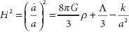
where H = Hubble parameter, a = scale factor, G = gravitational constant, ρ = mass density of universe, Λ = cosmological constant, K = curvature parameter, c = speed of light. By way of explanation, the scale factor, “a,” of the universe is a global multiplier to universe size. Imagine the universe as a perfectly laid out city with streets that travel only north-south and east-west. Streets are spaced at equal distance intervals. Street intersections then define perfectly symmetric city blocks. One could go further and think of buildings in the city as analogous with galaxies in the universe.

The distance from one city block to another is a function of two values: the originally laid out distance (call that the “normalized” distance) and the scale factor multiplier “a.” Note that, as in Fig. 1.1, when one multiplies by a scale factor of 1/2, one still has precisely the same city with the same number of city blocks. The only thing that has changed is the distance interval between the city blocks.

Now consider buildings within the city. If the city block distance were reduced to the size of buildings, clearly something must give. The buildings would be squeezed together and destroyed. This is analogous to what happens with matter in the real universe. The sizes of non-elementary mass structures such as protons, neutrons, atomic nuclei, and so on, are fixed; they do not change with the scale factor. Other physical structures, such as massless particles, do adjust with the scale factor. The wavelength of radiation adjusts and hence would gain (in the case of contraction) or lose (in the case of expansion) energy as a result.² When one crowds these particles in upon themselves, one will see a transition to different physics.

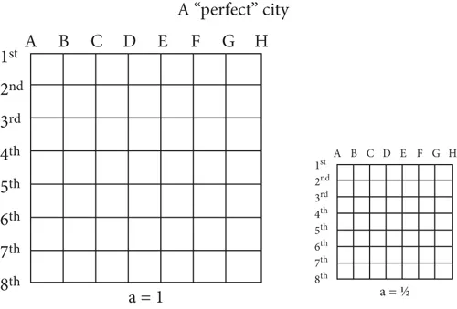
Figure 1.1 Analogy of the universe as a city laid out in a grid.

Recall that the full city is always present regardless of the value of the scale factor. So now consider two additional situations. First, suppose that the scale factor were to shrink to zero. Space (and time) would disappear. Any structure that could not transform to zero size would be destroyed. If there were no physical process that would allow such a thing to happen, we should seem to have a paradox. Either there must be an undiscovered physical process or the scale factor cannot, in reality, assume a null value.

Second, imagine that the city is of infinite size. Conceptually, there is no problem with extending the streets north-south and east-west to infinity in each direction. What does it mean to scale the universe’s size in such a situation? No matter what scale factor one adopts, the size of the universe remains infinite. Nevertheless, the idea of scaling still retains coherency in that we can apply a multiplier to the finite distance between city blocks. Yet what would be the meaning of applying a zero scale factor in this situation? Now it would appear that the size of the full universe is “zero times infinity” which, in general, can be any finite number (Barrow 2005, p. 160). What does this mean, given that the distance between any spot in the universe to any other spot must still be zero? GR simply breaks down at zero scale factor.

Whether or not the full universe is of infinite or finite size is given in the Friedmann equation by the curvature parameter “K.” A positive K indicates that the universe, much like the surface of the Earth, is unbounded yet of finite size. Going back to the analogy, imagine that the city is laid out over Earth’s entire curved surface. A traveler on 1st street would never come to the end; rather he would eventually come back to the location where he started. A positive K yields positive curvature and a closed universe. This is one type of “compact metric” within GR.

A zero value for “K” yields a “flat” universe. 1st street is unbounded and of infin ite length (in both directions). A similar situation obtains for a negative K value. Here one has negative, or “saddle-shaped” curvature. Two travelers moving east and side-by-side up 1st and 2nd streets would actually get laterally farther apart as the curvature of the surface causes the streets to diverge from each other. The latter case gives an infinitely sized “open” universe.

The components of the universe (all the energy, keeping in mind that E = mc2) determine what type of curvature the universe possesses. The “strength” of gravity, included in the equation via the parameter “G,” affects the magnitude of the curvature.

The parameters ρ and Λ indicate the type and magnitude of the different types of energy that cause the curvature. The parameter “ρ” represents the density (that is, the energy per unit volume) of the two types of “ordinary” energy: matter and radiation. It is “ordinary” in the sense that we are familiar with it in daily life and it is of a form that makes gravity an attractive force. Λ represents an exotic type of energy density which can transform gravity from an attractive to a repulsive force.

Friedmann’s first equation tells us how the scale factor changes as time elapses. Mathematically, this is the first derivative of the scale factor “a,” known as “a-dot,” or å. One can see that the increase (or decrease) in the scale factor is strongly a function of the universe’s energy content. Now the “ordinary” energy density ρ will become smaller as the universe expands, since one has the same amount of energy spread out over a greater volume. So its causal impact on the expansion will progressively diminish at ever later times (this works in reverse for contraction). By contrast, Λ, which represents the dark energy density, is constant. The dark energy does not become more dilute during expansion or concentrated during contraction. Hence, early in the life of an expanding universe Λ is unimportant compared to ρ. But its impact “snowballs” as time goes on. As long as the impact of ρ in the early universe is not enough to overturn an expansion and begin a contraction, the effect of Λ will eventually lead to a runaway expansion of the universe. There will appear a moment in the history of the universe when the dark energy will begin to dominate the ordinary energy, and the universe’s expansion will begin to accelerate. Recent observations, in fact, seem to show precisely this effect in our own universe, with a transition age at 9 billion years (Overbye 2006).

Friedmann’s second equation gives the rate of change of the expansion rate:

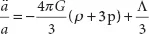
It determines whether the expansion itself is slowing or accelerating. This acceleration is referred to as “a-double-dot,” or ä. A new term “p” appears in the equation. This is the pressure (similar to the pressure of a gas inside a balloon). Pressure itself can produce gravitational force. Pressure is normally negligible for ordinary matter, although it can play a role in radiation dominated universes. Pressure, however, can have a tremendous impact given a universe dominated by dark energy. As Friedmann’s second equation shows, the rate at which the expansion of the universe accelerates is proportional to: (- µ - 3p). But the pressure in the vacuum is just equal to the negative of the energy density; this is called the equation of state. Hence, overall, the acceleration is positive (which will produce expansion) and proportional to twice the energy density.

Ordinary matter will exert positive pressure (which will keep a balloon inflated, for example). This type of pressure will produce an attractive gravitational force, which supplements the attractive gravity that accrues from mass. Dark energy has the bizarre property that it generates negative pressure. But dark energy, while it has a positive energy density (which contributes to attractive gravity) will, on net, produce a repulsive gravitational effect. Looking at Friedmann’s second equation, one sees that an attractive gravitational contribution tends to slow down expansion (or accelerate contraction), while repulsive gravity will do the opposite.

The monumental significance of the Friedmann-Lemaître model lay in its historization of the universe. As one commentator has remarked, up to this time the idea of the expansion of the universe “was absolutely beyond comprehension. Throughout all of human history the universe was regarded as fixed and immutable and the idea that it might actually be changing was inconceivable” (Naber 1988,pp. 126–27). But if the Friedmann-Lemaître model is correct, the universe can no longer be adequately treated as a static entity existing, in effect, timelessly. Rather the universe has a history, and time will not be a matter of indifference for our investigation of the cosmos.

In 1929 the American astronomer Edwin Hubble showed that the red-shift in the optical spectra of light from distant galaxies was a common feature of all measured galaxies and was proportional to their distance from us (Hubble 1929, pp. 168–73). This red-shift, first observed by Vesto Slipher at the Lowell Observatory,³ was taken to be a Doppler effect indicative of the recessional motion of the light source in the line of sight. Incredibly, what Hubble had discovered was the isotropic expansion of the universe predicted by Friedmann and Lemaître on the basis of Einstein’s GR. It was a veritable turning point in the history of science. “Of all the great predictions that science has ever made over the centuries,” exclaims John Wheeler, “was there ever one greater than this, to predict, and predict correctly, and predict against all expectation a phenomenon so fantastic as the expansion of the universe?” (Wheeler 1980, p. 354).

2.31 The standard hot Big Bang model

According to the Friedmann-Lemaître model, as time proceeds, the distances separating the ideal particles of the cosmological fluid constituted by the matter and energy of the universe become greater. It is important to appreciate that as a GR-based theory, the model does not describe the expansion of the material content of the universe into a pre-existing, empty, Newtonian space, but rather the expansion of space itself. The ideal particles of the cosmological fluid are conceived to be at rest with respect to space but to recede progressively from...

Table of contents

• Cover
• Half-Title
• Series
• Title
• Contents
• Acknowledgements
• Foreword
• Introduction Paul Copan
• 1 The Kalām Cosmological Argument: “Science” Excerpt William Lane Craig and James D. Sinclair
• 2 Why the Big Bang Singularity Does Not Help the Kalām Cosmological Argument for Theism J. Brian Pitts
• 3 On Non-Singular Spacetimes and the Beginning of the Universe William Lane Craig and James D. Sinclair
• 4 The Beginning of the Universe Alexander Vilenkin
• 5 A Dying Universe: The Long-Term Fate and Evolution of Astrophysical Objects Fred C. Adams and Gregory Laughlin
• 6 Heat Death in Ancient and Modern Thermodynamics Gábor Kutrovátz
• 7 Entropy and Eschatology: A Comment on Kutrovátz’s Paper “Heat Death in Ancient and Modern Thermodynamics” Milan M. Ćirković
• 8 The Generalized Second Law Implies a Quantum Singularity Theorem Aron C. Wall
• conclusion Therefore, the Universe Has a Cause
• Permissions
• Index
• Copyright