Smoothed Particle Hydrodynamics: A Meshfree Particle Method

A Meshfree Particle Method

G R Liu, M B Liu

• Publisher: WSPC
• Year: 2003
• ISBN:
  9789814365574
• Topic: Technology & Engineering
• Subtopic: Mechanical Engineering
• Index: Technology & Engineering

This is the first-ever book on smoothed particle hydrodynamics (SPH) and its variations, covering the theoretical background, numerical techniques, code implementation issues, and many novel and interesting applications.

It contains many appealing and practical examples, including free surface flows, high explosive detonation and explosion, underwater explosion and water mitigation of explosive shocks, high velocity impact and penetration, and multiple scale simulations coupled with the molecular dynamics method. An SPH source code is provided, making this a friendly book for readers and SPH users.

Supplementary Materials
Software

Contents:

• SPH Concept and Essential Formulation
• Constructing Smoothing Functions
• SPH for General Dynamic Fluid Flows
• Discontinuous SPH (DSPH)
• SPH for Simulating Explosions
• SPH for Underwater Explosion Shock Simulation
• SPH for Hydrodynamics with Material Strength
• Coupling SPH with Molecular Dynamics for Multiple Scale Simulations
• Computer Implementation of SPH and a 3D SPH Code

Readership: Researchers, practitioners, upper-level undergraduates, graduate students, and academics in computational mechanics and engineering.

Chapter 1

---

Introduction

---

1.1 Numerical simulation

1.1.1 Role of numerical simulation

Numerical simulation using computers or computational simulation has increasingly become a very important approach for solving complex practical problems in engineering and science. Numerical simulation translates important aspects of a physical problem into a discrete form of mathematical description, recreates and solves the problem on a computer, and reveals phenomena virtually according to the requirements of the analysts. Rather than adopting the traditional theoretical practice of constructing layers of assumptions and approximations, this modern numerical approach attacks the original problems in all its detail without making too many assumptions, with the help of the increasing computer power.

Numerical simulation provides an alternative tool of scientific investigation, instead of carrying out expensive, time-consuming or even dangerous experiments in laboratories or on site. The numerical tools are often more useful than the traditional experimental methods in terms of providing insightful and complete information that cannot be directly measured or observed, or difficult to acquire via other means.

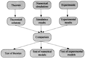
Numerical simulation with computers plays a valuable role in providing a validation for theories, offers insights to the experimental results and assists in the interpretation or even the discovery of new phenomena. It acts also as a bridge between the experimental models and the theoretical predictions as schematically shown in Figure 1.1.

Figure 1.1 Connection between the numerical simulations, theories and experiments. The connection is very important in conducting scientific investigations. In the connection, the numerical simulation is playing an increasingly important role.

1.1.2 Solution procedure of general numerical simulations

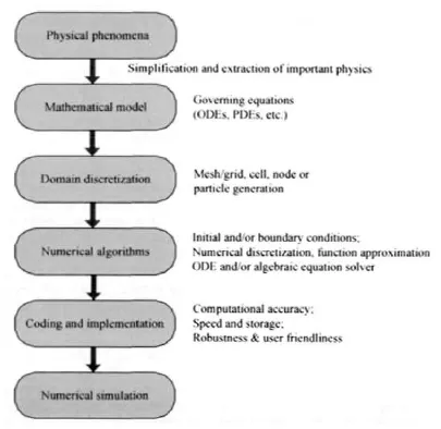
Numerical simulations follow a similar procedure to serve a practical purpose. There are in principle some necessary steps in the procedure, as shown in Figure 1.2. From the physical phenomena observed, mathematical models are established with some possible simplifications and assumptions. These mathematical models are generally expressed in the form of governing equations with proper boundary conditions (BC) and/or initial conditions (IC). The governing equations may be a set of ordinary differential equations (ODE), partial differential equations (PDE), integration equations or equations in any other possible forms of physical laws¹. Boundary and/or initial conditions are necessary for determining the field variables in space and/or time.

To numerically solve the governing equations, the involved geometry of the problem domain needs to be divided into discrete components. The domain discretization techniques may be different for different numerical methods. Domain discretization usually refers to representing a continuum problem domain with a finite number of components, which form the computational frame for the numerical approximation. The computational frame is traditionally a set of mesh or grid, which consists of a lattice of points, or grid nodes to approximate the geometry of the problem domain. The grid nodes are the locations where the field variables are evaluated, and their relations are defined by some kind of nodal connectivity. Grid nodes are connected to form a mesh following the connectivity. Accuracy of the numerical approximation is closely related to the mesh cell size and the mesh patterns.

Figure 1.2 Procedure of conducting a numerical simulation.

Numerical discretization provides means to change the integral or derivative operations in the governing equations in continuous forms to discrete representations. It is closely related to the domain discretization technique applied. The numerical discretization is based on a theory of function approximations (Liu, 2002). After domain discretization and numerical discretization, the original physical equations can be changed into a set of algebraic equations or ordinary differential equations, which can be solved using the existing numerical routines. In the process of establishing the algebraic or ODE equations, the so-called strong or weak form formulation can be used (see, e.g., Liu, 2002). As recently reported by Liu and Gu (2002, 2003), these two forms of formulation can also be combined together to take the fullest advantages of both weak and strong form formulations. This combination led to the development of the meshfree weak-strong (MWS) form methods.

Implementation of a numerical simulation involves translating the domain decomposition and numerical algorithms into a computer code in some programming language(s). In coding a computer program, the accuracy, and efficiency (speed and storage) are two very important considerations. Other considerations include robustness of the code (consistency check, error trap), user-friendliness of the code (easy to read, use and even to modify), etc. Before performing a practical numerical simulation, the code should be verified to reproduce sets of experimental data, theoretical solutions, or the exact results from other established methods for benchmark problems or actual engineering problems.

For numerical simulations of problems in fluid mechanics, the governing equations can be established from the conservation laws, which states that a certain number of system field variables such as the mass, momentum and energy must be conserved during the evolution process of the system (see, Chapter 4 for details). These three fundamental principles of conservation, together with additional information concerning the specification of the nature of the material/medium, conditions at the boundary, and conditions at the initial stage completely determine the behavior of the fluid system². These fundamental physical principles can be expressed in the form of some basic mathematical equations called governing equations. In most circumstances the governing equations are partial differential equations (PDE).

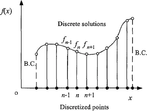
Except for a few circumstances, it is very difficult to obtain analytical solution of these integral equations or partial differential equations. Computational fluid dynamics (CFD) deals with the techniques of spatially approximating the integral or the differential operations in the integral or differential equations with the discretized counterparts that are usually in a form of simple algebraic summation. This approximation leads to a set of algebraic equations (or ODEs with respect to time only) that can be solved to obtain numerical values for field functions (such as density, pressure, velocity, etc.) at discrete points in space and/or time (Figure 1.3). A typical numerical simulation of a CFD problem involves the following factors.

1. governing equations,

2. proper boundary conditions and/or initial conditions,

3. domain discretization technique,

4. numerical discretization technique,

5. numerical technique to solve the resultant algebraic equations or ordinary differential equations (ODE).

Figure 1.3 Domain and numerical discretization for a numerical simulation of a field function f(x) defined in one-dimensional space.

---

1.2 Grid-based methods

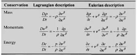
There are two fundamental frames for describing the physical governing equations: the Eulerian description and the Lagrangian description. The Eulerian description is a spatial description, and is typically represented by the finite difference method (FDM) (see, e.g., Anderson, 1995; Hirsch, 1988; Wilkins, 1999). The Lagrangian description is a material description, and is typically represented by the finite element method (FEM) (see, e.g., Zienkiewicz and Taylor, 2000; Liu and Quek, 2003, etc.). For example, in fluid mechanics, if the viscosity and the heat conduction as well as the external forces are neglected, the conservation equations in PDE form for these two descriptions are very much different, as listed in Table 1.1.

Table 1.1 Conservation equations in PDE form in the Lagrangian and Eulerian descriptions

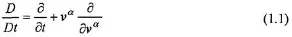
In Table 1.1, ρ, e, ν and x are density, internal energy, velocity and position vector respectively. The Greek superscripts α and β are used to denote the coordinate directions, while the summation in the equations is taken over repeated indices. It is seen that the differences between the two sets of equations are inherited in the definition of the total time derivative as the combination of the local derivative and the convective derivative, i.e.,

where D/Dt is the total time derivative (or substantial derivative, material derivative, or global derivative) that is physically the time rate of change following a moving fluid elements;

is the local derivative that is physically the time rate of change at a fixed point;

is the convective derivative that is physically the change due to the movement of the fluid element from one location to another in the flow field where the flow properties are spatially different. Therefore, the total time derivative describes that the flow property of the fluid element is changing, as a fluid element sweeps passing a point in the flow. This is because 1) at that point, the flow field property itself may be fluctuating with time (the local derivative); 2) the fluid element is on its way to another location in the flow field where the flow property may be different (the convective derivative).

The Eulerian and Lagrangian descriptions correspond to two disparate kinds of grid of domain discretization: the Eulerian grid and the Lagrangian grid. Both of them are widely used in numerical methods with preferences on types of problems, and hence are briefed in the following.

1.2.1 Lagrangian grid

In the Lagrangian grid-based methods such as the well-known and widely used FEM (see, e.g., Zienkiewicz and Taylor, 2000; Liu and Quek, 2003; etc.), the grid is fixed to or attached on the material in the entire computation process, and therefore it moves with the material as illustrated in Figure 1.4.

Figure 1.4 Lagrangian mesh/cells/grids for a shaped charge detonation simulation. The triangular cells and the entire mesh of cell move with the material.

Since each grid node follows the path of the material at the grid point, the relative movement of the connecting nodes may result in expansion, compression and deformation of a mesh cell (or element). Mass, momentum and energy are transported with the movement of the mesh cells. Because the mass within each cell remains fixed, no mass flux crosses the mesh cell boundaries. When the material deforms, the mesh deforms accordingly.

The Lagrangian grid-based methods have several advantages.

1. Since no convective term exists in the related partial differential equations, the code is conceptually simpler and should be faster as no computational effort is necessary for dealing with the convective terms.

2. Since the grid is fixed on the moving material, the entire time history of all the field variables at a material point can be easily tracked and obtained.

3. In the Lagrangian computation, some grid nodes can be placed along boundaries and material interfaces. The boundary conditions at free surfaces, moving boundaries, and material interfaces are automatically imposed, tracked and determined simply by the movement of these grid nodes.

4. Irregular or complicated geometries can be conveniently treated by using an irregular mesh.

5. Since the grid is required only within the problem domain, no additional grids beyond the problem domain is required, and hence the Lagrangian grid-based methods are computationally efficient.

Due to these advantages, Lagrangian methods are very popular and successful in solving computational solid mechanics (CSM) problems, where the deformation is not as large as that in the fluid flows.

However, Lagrangian grid-based methods are practically very difficult to apply for cases with extremely distorted mesh, because their formulation is always based on mesh. When the mesh is heavily distorted, the accuracy of the formulation and hence the solution will be severely affected. In addition, the time step, which is controlled by the smallest element size, can become too small to be efficient for the time marching, and may even lead to the breakdown of the computation.

A possible option to enhance the Lagrangian computation is to rezone the mesh or re-mesh the problem domain. The mesh rezoning involves overlaying of a new, undistorted mesh on the old, distorted mesh, so that the following-up computation can be perform...

Table of contents

• Cover Page
• Title Page
• Copyright Page
• Dedication Page
• The Authors
• Contents
• Preface
• 1 - Introduction
• 2 - SPH Concept and Essential Formulation
• 3 - Constructing Smoothing Functions
• 4 - SPH for General Dynamic Fluid Flows
• 5 - Discontinuous SPH (DSPH)
• 6 - SPH for Simulating Explosions
• 7 - SPH for Underwater Explosion Shock Simulation
• 8 - SPH for Hydrodynamics with Material Strength
• 9 - Coupling SPH with Molecular Dynamics for Multiple Scale Simulations
• 10 - Computer Implementation of SPH and a 3D SPH Code
• Bibliography
• Index