One Hundred Physics Visualizations Using MATLAB

Dan Green

• Publisher: WSPC
• Year: 2013
• ISBN:
  9789814518468
• Topic: Physical Sciences
• Subtopic: Mathematical & Computational Physics

This book provides visualizations of many topics in general physics. The aim is to have an interactive MATLAB script wherein the user can vary parameters in a specific problem and then immediately see the outcome by way of dynamic “movies” of the response of the system in question. MATLAB tools are used throughout and the software scripts accompany the text in Symbolic Mathematics, Classical Mechanics, Electromagnetism, Waves and Optics, Gases and Fluid Flow, Quantum Mechanics, Special and General Relativity, and Astrophysics and Cosmology. The emphasis is on building up an intuition by running many different parametric choices chosen actively by the user and watching the subsequent behavior of the system.

Physics books using MATLAB do not have the range — or the intent — of this text. They are rather steeped in technical detail. Symbolic math is used extensively and is integral to the aim of using MATLAB tools to accomplish the technical aspects of problem solving.

Contents:

• Symbolic Mathematics and Math Tools
• Classical Mechanics
• Electromagnetism
• Waves and Optics
• Gases and Fluid Flow
• Quantum Mechanics
• Special and General Relativity
• Astrophysics and Cosmology

Readership: Graduate students and researchers in physics.

Chapter 1

Symbolic Mathematics and Math Tools

“If people do not believe that mathematics is simple, it is only because they do not realize how complicated life is.”

— John von Neumann

“Pure mathematics is, in its way, the poetry of logical ideas.”

— Albert Einstein

“There cannot be a language more universal and more simple, more free from errors and obscurities . . . more worthy to express the invariable relations of all natural things [than mathematics]. [It interprets] all phenomena by the same language, as if to attest the unity and simplicity of the plan of the universe.”

— Joseph Fourier

1.1. MATLAB Functions

The first section will deal with mathematical tools, mostly using the MATLAB symbolic math package. Although not strictly physics, the tools of mathematics are crucial because they are the language of physics and physics cannot be understood well without a facility in that language. Some of these tools will be invoked later in the more physics oriented demonstrations found in the following sections.

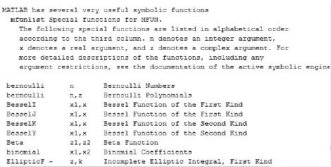
MATLAB has a very large suite of special functions which are available to the user. They can be found for the MAPLE symbolic functions, by invoking the command “mfunlist”. The first page of symbolic functions is shown in Figure 1.1.

The complete set of MATLAB functions is available using the HELP tab in the Command Window. The sequence is HELP/ MATLAB/functions. There are ten headings under functions and by using them all, the MATLAB functions are available for examination. There are two other useful headings, examples and demos, which give useful aid in understanding some applications of these functions.

Figure 1.1: First entries for MATLAB symbolic functions.

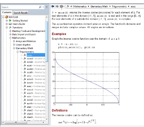
Specific descriptions and examples follow when the help function is explicitly queried. One of the strengths of MATLAB is that there are so many supported special functions and that they are described using the help files. These utilities make the use of these functions quite transparent. An example is given in Figure 1.2, where the path to drill down the function tree to “acos” is shown.

A full list is invoked using the .m script “MATLAB_Functions” in the Command Window, which gives the complete list of symbolic functions and also prints the path to retrieve all the MATLAB numerical special functions. Tools that are useful with symbolic math are: “sym”, “factor”, “simplify”, “pretty”, “simple” and “eval”. These tools can be used to simplify the symbolic strings and “eval” is used to convert them for numerical evaluations.

1.2. Symbolic Differentiation

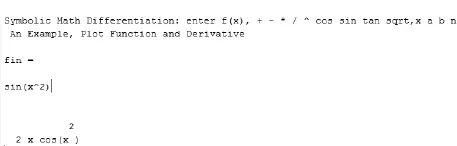
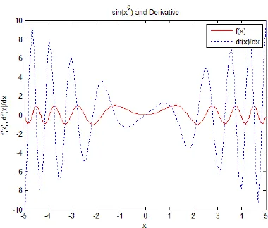
A first demonstration of the use of symbolic math is to evaluate derivatives. As with most of the demonstrations in this text, there is a recurring format. First, explanatory text is printed by invoking “help” in the script, an example is given, and then there is a menu driven prompt which asks the user to try other functions or additional options. The example is plotted in order to see the result of the operations. The MATLAB script “diff” is the core of the script “SM_Diff”. The plot of the printout of the example is shown in Figure 1.3, while the function and derivative is shown in Figure 1.4. Most of the exercises have explanatory printout as the initial response to starting the specific script. The format of the script used in this text is made as uniform as possible within the different physics being explored so as to make the script easy to use, understand, and ultimately be modified by the users to follow their interests.

Figure 1.2: Result of using the help facility to find the description of the acos function.

1.3. Symbolic Integration

A similar script performs symbolic integration, with an example followed by possible user input functions with resulting plots. The example provided is shown in Figure 1.5. The script, “SM_Int” is set up to perform indefinite integrals. However, MATLAB has other options using the “int” script, such as defining the variable not to be x, but a user defined variable or supplying the limits for a definite integral. The reader is encouraged to further explore the available options in MATLAB should they be interested in using the “int” function in greater depth. Invoking “help int” in the Command Window yields examples and options for symbolic integration. In particular, all of the symbolic functions indicated in Figure 1.1 are available as integrand candidates.

Figure 1.3: Printout for the symbolic differentiation script.

Figure 1.4: Plot of the example function and the derivative. Other functions can be input by the user in symbolic form as often as is desired in one session of the script use.

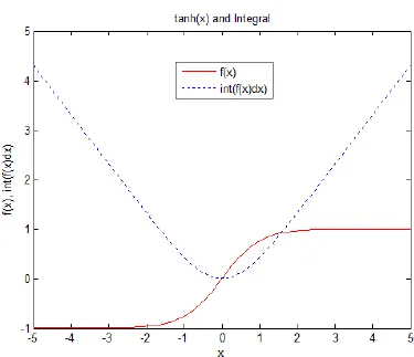
Figure 1.5: Example for the symbolic integration of tanh(x) as an indefinite integral.

1.4. Taylor Expansion

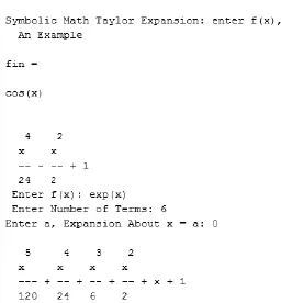
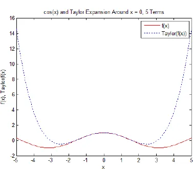
Power law expansions are useful tools in several applications. They are available using the MATLAB function “taylor”, where the expansion point and the number of terms in the series can be selected. The printout from the script “SM_Taylor” for the example and the menu for the user are shown in Figure 1.6. The plotting output for the example expansion is given in Figure 1.7. Clearly, an intuition can be built up fairly quickly as to the domain of validity of the expansion as to how well it approximates the function. It is clear that the expansion of the cos function with five terms is a fair representation for |x| < 2. As with other MATLAB scripts, a full description is available from the Command Window via the help query or using the help tab.

The user chooses the function, the number of terms, and the offset, or expansion point in the variable x. The results are displayed graphically in the figure. That figure can be printed or edited using the Figure Window and the editing tabs supplied in that window.

Figure 1.6: Printout for the “SM_Taylor” script with the example of cos(x) and the menu choice of exp(x).

Figure 1.7: Example from the “SM_Taylor” script for the Taylor expansion of cos(x).

1.5. Series Summation

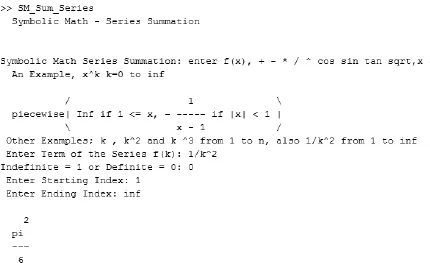
There is the ability in MATLAB to symbolically sum a series using the “symsum” script. This script has been used with a wrapper script called “SM_Sum_Series”. An example and a user input series is shown in Figure 1.8. As always, a user driven menu is provided so that any series can be input and summed. More details and other examples can be accessed with the input “help symsum” in the Command Window.

Figure 1.8: Output of the series summing script for an example and then for a user defined series with the terms being possibly definite or indefinite.

1.6. Polynomial Factorization

Polynomials can be factorized symbolically. The script “factor” is used in the wrapper script, “SM_Factor” and an example with user input is shown in Figure 1.9. Numbers can also be factored.

1.7...

Table of contents

• Cover
• Halftitle
• Title
• Copyright
• Dedication
• Preface
• Contents
• 1. Symbolic Mathematics and Math Tools
• 2. Classical Mechanics
• 3. Electromagnetism
• 4. Waves and Optics
• 5. Gases and Fluid Flow
• 6. Quantum Mechanics
• 7. Special and General Relativity
• 8. Astrophysics and Cosmology
• Appendix — Script for Classical Mechanics
• References
• Index