Current at the Nanoscale

An Introduction to Nanoelectronics

Colm Durkan

• Publisher: WSPC
• Year: 2013
• ISBN:
  9789814579124
• Edition: 2
• Topic: Technology & Engineering
• Subtopic: Electrical Engineering & Telecommunications
• Index: Technology & Engineering

This second edition of the book, initially written as an introductory text dealing with how electric currents behave at the nanometer scale, begins with a general description of electric currents at the macroscale. Then by considering the physical length scales relevant to electron flow, it is observed how the behavior of currents varies as they approach the nanoscale. A quantum description of electric current is covered as well as its relevance, with particular reference to defects, grain boundaries, tunnelling and atomic contacts, followed by the effects of current flow through nanostructures, including electromigration, of particular relevance for transistor miniaturization. Next, the techniques used to probe currents and voltages at the nanoscale are considered, focusing on scanning-probe microscopy and transport measurements, before considering electronic transport through molecular and single-electron devices.

The book will tie together several aspects of current and recent research on the current flow at the nanoscale. Due to the introductory nature of the book, it will not become obsolete quickly, and chapters can be added at will at later stages as new developments arise.

Contents:

• Macroscopic Current Flow
• Quantum Current Flow
• Mesoscopic Transport: Between the Nanoscale and the Macroscale
• Scanning-Probe Multimeters
• Electromigration: Current-Induced Damage
• Elements of Single-Electron and Molecular Electronics

Readership: Advanced undergraduates, graduate students and researchers in nanotechnology.

Chapter 1

Macroscopic Current Flow

Nanotechnology has been a topic arousing much interest for over a decade now, and is starting to deliver on its initial promise. The reason for this sustained interest is that when materials have features that are only a few nm across (a nm is one nanometer which is 1 billionth of a meter, and Nano comes from the Greek “Nanos”, meaning dwarf), their physical (electrical, magnetic, mechanical, optical and chemical) properties start to become very sensitive to size and shape and can to a large extent be controlled, to create novel functionality. Transistors are already at the scale of ~ 20 nm, and are starting to display electrical characteristics that deviate from their classically expected ones — hence the need for this book.

In order to be able to gain any insight into current flow at the nanometer scale, which we will refer to from now on as the nanoscale, we must first consider what happens at macroscopic scales and then see the effect of reducing the dimensions to the nanoscale. The behaviour of conventional electrical circuits can be understood in quite simple terms, whereas at the nanoscale, there are a number of subtle effects that can only be understood within the framework of quantum mechanics, as we shall see in this chapter and in Chapter 2. In between these disparate regimes, we have mesoscopic transport, which we will briefly consider in Chapter 3.

On the basis of his detailed experimental observations in the 1820s, Georg Ohm formulated his well-known law [1] stating the following:

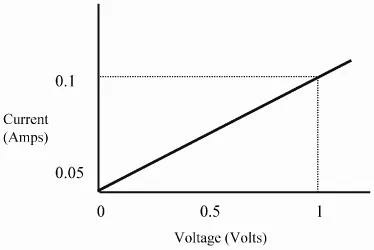
For a constant temperature, the current flowing through a conductor is directly proportional to the potential difference between its ends. Or, V = IR.

This is illustrated in Fig. 1.1. The constant of proportionality between applied voltage and the resulting current is known as resistance, R. The resistance depends on the geometry of the conductor and a material constant — resistivity as R = ρl/A, where l and A are the length and cross-sectional area of the conductor, respectively. As we will see later, when any of the dimensions of a conductor are shrunk to the nanoscale, resistivity itself becomes strongly dependent on geometry, and is no longer just a number. For now however, let us consider Ohm’s law in more detail, from a purely classical (i.e. non-quantum) standpoint — Drude’s model of electronic conduction.

Fig. 1.1. Relationship between current and voltage for a conductor. In this case the resistance is 10 Ω (i.e. V =10I ).

We will then introduce the necessary corrections that must be made to be consistent with quantum mechanics which comes to the fore at small length scales. We will consider the following questions central to the flow of electric current:

1. What is electric current?

2. Why and how does current depend on voltage?

3. What are typical values of resistance/resistivity of conductors, and what do they depend on?

4. How does resistance depend on temperature, and why?

5. Why are some materials conductors, and others semiconductors or insulators?

1.1 The Classical (Drude) Model of Electronic Conduction and Ohm’s Law

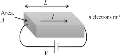
To answer the above questions, we need to consider what happens when we apply a voltage, V, to a conductor. The voltage produces an electric field E, across the conductor, as illustrated in Fig. 1.2. This electric field induces a force on the electrons (of charge, e = −1.6×10⁻¹⁹ C) of strength eE, in a direction opposite to that of the applied field (as the electron charge is negative). On this basis, we would therefore expect the electrons to continue to accelerate as they traverse the conductor (cf. Newton’s second law). This flow of charge carriers within a conductor is known as a current, I, and the magnitude of the current in a given direction is the amount of charge (in Coulombs) passing a point in the conductor per second. A current of 1 A (Ampere or Amp) corresponds to 3.25 ×10¹⁸ electrons passing a point per second.

Fig. 1.2. Schematic showing current, I, due to a voltage, V, applied to a conductor of length L and cross-sectional area, A. The current, I is defined as the amount of charge per unit time passing a point, which is the number of electrons per unit volume, n, multiplied by the volume, A × L , divided by the time taken to transit the distance, L. This is nAve, where v is the average velocity, or drift velocity of the electrons.

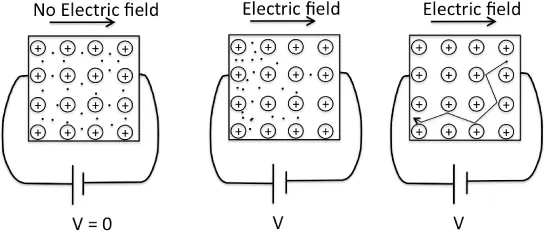
Fig. 1.3. The flow of charge in a conductor under an applied electric field, E. On the left, with no voltage applied, the electrons diffuse randomly around, then with a voltage applied, the electrons migrate against the electric field. Considering a single electron, its average motion is along the direction of the electric field, but this is made up of a series of directed random walks each of average length ℓ (the mean free path). The average velocity is indicated by the dotted line in the figure on the right, showing how the velocity varies between and during scattering events.

In reality, we know that electrons do not accelerate indefinitely as they flow through a conductor, but they drift along at a finite, and generally rather slow speed (called the drift velocity, typically a few mm.s⁻¹ in a good conductor, which is orders of magnitude smaller than the Fermi velocity of the electrons, typically ~10⁶ m.s⁻¹ ). This drift velocity is analogous to the terminal velocity experienced by falling objects (which continually lose momentum to air molecules), and is due to the electrons colliding with other electrons, impurities, lattice imperfections and lattice vibrations (phonons) within the conductor. The average...

Table of contents

• Cover
• Half Title
• Title Page
• Copyright
• Dedication
• Preface to Second Edition
• Preface to First Edition
• Contents
• 1. Macroscopic Current Flow
• 2. Quantum Current Flow
• 3. Mesoscopic Transport: Between the Nanoscale and the Macroscale
• 4. Scanning-Probe Multimeters
• 5. Electromigration: Current-Induced Damage
• 6. Elements of Single-Electron and Molecular Electronics
• Solutions to Problems
• Index