Causality, Correlation And Artificial Intelligence For Rational Decision Making

Tshilidzi Marwala

• Publisher: WSPC
• Year: 2015
• ISBN:
  9789814630887
• Topic: Sciences biologiques
• Subtopic: Science générale

Causality has been a subject of study for a long time. Often causality is confused with correlation. Human intuition has evolved such that it has learned to identify causality through correlation. In this book, four main themes are considered and these are causality, correlation, artificial intelligence and decision making. A correlation machine is defined and built using multi-layer perceptron network, principal component analysis, Gaussian Mixture models, genetic algorithms, expectation maximization technique, simulated annealing and particle swarm optimization. Furthermore, a causal machine is defined and built using multi-layer perceptron, radial basis function, Bayesian statistics and Hybrid Monte Carlo methods. Both these machines are used to build a Granger non-linear causality model. In addition, the Neyman–Rubin, Pearl and Granger causal models are studied and are unified. The automatic relevance determination is also applied to extend Granger causality framework to the non-linear domain. The concept of rational decision making is studied, and the theory of flexibly-bounded rationality is used to extend the theory of bounded rationality within the principle of the indivisibility of rationality. The theory of the marginalization of irrationality for decision making is also introduced to deal with satisficing within irrational conditions. The methods proposed are applied in biomedical engineering, condition monitoring and for modelling interstate conflict.

Contents:

• Introduction to Artificial Intelligence based Decision Making
• What is a Correlation Machine?
• What is a Causal Machine?
• Correlation Machines Using Optimization Methods
• Neural Networks for Modeling Granger Causality
• Rubin, Pearl and Granger Causality Models: A Unified View
• Causal, Correlation and Automatic Relevance Determination Machines for Granger Causality
• Flexibly-bounded Rationality
• Marginalization of Irrationality in Decision Making
• Conclusions and Further Work

Readership: Graduate students, researchers and professionals in the field of artificial intelligence.
Key Features:

• It proposes fresh definition of causality and proposes two new theories i.e. flexibly bounded rationality and marginalization of irrationality theory for decision making
• It also applies these techniques to a diverse areas in engineering, political science and biomedical engineering

Chapter 1

Introduction to Artificial Intelligence based Decision Making

Abstract.In this chapter, decision making which is based on causality, correlation and artificial intelligence is introduced. The concept of correlation is introduced and is applied to build a correlation function. Furthermore, it relates causality to correlation and uses it to build a causal function. Artificial intelligence methods are introduced and these include neural networks, particle swarm optimization, genetic algorithm and simulated annealing. It describes decision making and outlines the rest of the book.

1.1 Introduction

The problem of understanding causality has pre-occupied philosophers for a very long time. From the times of Plato and Aristotle and even before that period, mankind has been asking why and how they are on this planet and various answers to these questions involve causality. The very idea that a higher being, or a great architect of the universe created, mankind is squarely premised on the principle of causality. The significance of understanding causality to satisfy human curiosity and enhance the functioning of society is enormous. As an example, the medical field is based on the premise that some medicines cause healing of diseases. To link specific medicines to the curing of diseases requires a good understanding of causality and as long as this understanding is not complete the results of clinical studies will always be sub-optimal. One example to illustrate this, is the avocado pear that was thought to be dangerous because the causal relation between avocado pear consumption and cholesterol was poorly understood but today it is considered good for one’s cholesterol.

There is an old Tshivenda saying that states: “Tsho bebiwaho tsho fa” (Marwala, 2013a). What this expression signifies is that there is a perfect correlation between birth and death and those who are born will necessarily die. Many have simplified and misinterpreted this allegory to purport that it alludes to the fact that birth causes death. In fact, there is an information flow from birth to death but this is not causal information. It might be that the actual causal relation for this case was between a road accident and death, therefore, the road accident caused death. This example illustrates a very simple explanation of what a cause is and what a correlation is. On trying to understand causality, it is vital to understand the principle of correlation because within any causal model lies a correlation function.

1.2 Correlation

In this section, we explore the concept of correlation, what it is and what it can be used for. To illustrate this, we invoke the relationship between obesity and heart attack. In this example, the two variables x indicating a person’s weight and y indicating whether they had a heart attack. In this case, variable x is positively correlated to variable y.

1.2.1 What is correlation?

According to www.dictionary.com correlation is defined as: “the degree to which two or more attributes or measurements on the same group of elements show a tendency to vary together.” This degree to which variables vary together can be quantified. Two variables are correlated if their underlying substructures are connected. For example, if one was to measure the heart rate and blood pressure of patient John, then these parameters may be correlated primarily because they are measurements from a common structure, and in this case a patient called John. In statistics this case is known as confounding.

1.2.2 Correlation function

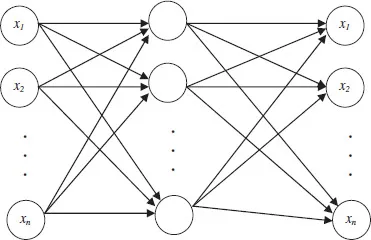
In this book, we introduce a concept called a correlation function which is a conventional predictive system that is primarily based on mapping variables to themselves and this is called the auto-associative network (Kramer, 1992). It is a process through which a system is able to recreate a complete set of information from a small piece of information. For example, one could easily complete the following statement if one is familiar with the former USA President J.F. Kennedy: “Ask not what your country can do for you but ….” In order to achieve this task, the auto-associative memory is used. The auto-associative networks are sometimes called auto-encoders or memory networks. These networks have been used in a number of applications including novelty detection, image compression (Rios and Kabuka, 1995) and missing data estimation (Marwala, 2009). An illustration of the auto-associative network is shown in Figure 1.1.

Masuda et al. (2012) successfully applied auto-associative memories based on recurrent neural networks to maximize the number of correctly stored patterns whereas Miranda et al. (2012) successfully applied auto-associative neural networks and mean shift for fault detection in power transformers. Valle and Grande Vicente (2011) successfully applied auto-associative networks to reconstruct color images corrupted by either impulsive or Gaussian noise, whereas Fernandes et al. (2011) successfully applied auto-associative pyramidal neural network for face verification, whereas Jeong et al. (2011) successfully applied auto-associative multilayer perceptron for laser spot detection based on computer interface system. Other successful applications of auto-associative network are in business failure (Chen, 2010) and gaze tracking (Proscevicius et al., 2010).

Figure 1.1 An auto-associative network

The principles governing the auto-associative network are as follows (Marwala, 2009):

1. A correct model that describes inter-relationships that exist amongst the data variables and define the rules that govern the data, is identified. This is achieved using an auto-associative memory network.

2. In order to estimate unknown variable(s), the correct estimated variable(s) are those that when identified they obey all the inter-relationships that exist amongst the data as defined in Step 1 and the rules that govern the data. In order to ensure that the estimated values obey the inter-relationships in the data, an optimization method that treats the unknown variable(s) as design variable(s) and the interrelationships amongst the data and rules that govern the data as the objective to be reached. Therefore, the unknown variable(s) estimation problem is fundamentally an optimization problem where the objective is to estimate unknown variable(s) by ensuring that the rules and inter-relationships governing the data are maintained.

3. It is vital to have a good idea of the bounds that govern the unknown variable(s) in order to aid the optimization process.

1.3 Causality

1.3.1 What is causality?

According to the Oxford English dictionary causality is defined as “the relationship between something that happens and the effect it produces” and defines a cause as “making something” while an effect is defined as “a change which is a result of an action”. The cause does not necessarily have to be one-dimensional. For example, in a causal relationship between sunlight, minerals, air and water causing the tree to grow, the cause has 4 dimensions (sunlight, minerals, air and water). This book adopts the concept that for one variable to cause another, there has to be a flow of information from the cause to the effect. According to Suppes (1970), there are many different types of causes and these are prima facie causes, spurious causes, direct causes, supplementary causes, sufficient causes and negative causes.

According to Suppes (1970), the event B is the prima facie cause of event A if event A happened after event B has happened, the probability of event B happening p(B) is greater than zero and the probability of event A happening given the fact that event B has happened p(A|B) is greater than the probability of event A happening p(A). Spurious cause is the cause of an event in which an earlier cause is the real cause of the event. According to Suppes (1970), “an event B_t′ is a spurious cause of A_t if and only if t′ > t″ exists and that there is a partition π_t″ such that for all elements C_t″ of π_t″t′ < t, p(B_t′) > 0, p(A_t|B_t′) > p(A_t), p(B_t′C_t″) > 0 and p(A_t|B_t′C_t″) = p(A_t|C_t″).” Again according to Suppes (1970), “an event B_t′ is a direct cause of A_t if and only if B_t′ is a prima facie cause of A_t and there is no t″ and no partition π_t″ such that for every C_t″ in π_t″t′ < t″ < t, P(B_t′C_t″) > 0 and p(A_t|B_t′C_t″) = p(A_t|C_t″)”. Supplementary causes are more than one cause supplementing one another to cause an event. Suppes (1970) defines B_t′ and C_t″ as supplementary causes of A_t “if and only if B_t′ is a prima facie cause of A_t, C_t″ is a prima facie cause of A_t, p(B_t′C_t″) > 0, p(A|B_t′C_t″) > max(p(A_t|B_t′), p(A_t|C_t″)”. Sufficient causes are causes that cause the event to definitely happen. Accordingly, Suppes (1970) defines that “B_t′ is a sufficient cause of A_t if and only if B_t′ is a prima facie cause of A_t and p(A_t|B_t′) = 1”. Negative cause is an event that causes another event not to occur. According to Suppes (1970), “the event B_t′ is a prima facie negative cause of event A_t if and only if t′ < t, p(B_t′) > 0 and p(A_t|B_t′) < p(A_t).”

1.3.2 Theories of causality

In this chapter, we use key terminologies one of which is a causal path that links an event (cause) to another event (effect) as well as a correlation path which links one variable to another. Hume (1896) advanced the following eight principles of causality:

1. The cause and effect are connected in space and time.

2. The cause must happen before the effect.

3. There should be a continuous connectivity between the cause and the effect.

4. The specific cause must at all times give the identical effect, and the same effect should not be obtained from any other event but from the same cause.

5. Where a number of different object give the same effect, it ought to be because of some quality which is the same amongst them.

6. The difference in the effects of two similar events must come from that which they are different.

7. When an object changes its dimensions with the change of its cause, it is a compounded effect from the combination of a number of different effects, which originate from a number of different parts of the cause.

8. An object which occurs for any time in its full exactness without any effect, is not the only cause of that effect, but needs to be aided by some other norm which may advance its effect and action.

Pećnjak (2011) demonstrated that unlike what Hume proposed under particular scenarios the same causes can have very different effects whereas Paoletti (2011) studied causes as contiguous events. McBreen (2007) studied realism and empiricism in Hume’s account of causality and observed that the realist explanation ...

Table of contents

• Cover
• Halftitle
• Title Page
• Copyright Page
• Preface
• Acknowledgments
• Contents
• 1. Introduction to Artificial Intelligence based Decision Making
• 2. What is a Correlation Machine?
• 3. What is a Causal Machine?
• 4. Correlation Machines Using Optimization Methods
• 5. Neural Networks for Modeling Granger Causality
• 6. Rubin, Pearl and Granger Causality Models: A Unified View
• 7. Causal, Correlation and Automatic Relevance Determination Machines for Granger Causality
• 8. Flexibly-bounded Rationality
• 9. Marginalization of Irrationality in Decision Making
• 10. Conclusions and Further Work
• Index