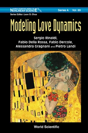
Modeling Love Dynamics

Sergio Rinaldi, Fabio Della Rossa, Fabio Dercole, Alessandra Gragnani, Pietro Landi

• Publisher: WSPC
• Year: 2015
• ISBN:
  9789814696333
• Topic: Biological Sciences
• Subtopic: Science General
• Index: Biological Sciences

This book shows, for the very first time, how love stories — a vital issue in our lives — can be tentatively described with classical mathematics. Focus is on the derivation and analysis of reliable models that allow one to formally describe the expected evolution of love affairs from the initial state of indifference to the final romantic regime. The models are in full agreement with the basic philosophical principles of love psychology. Eight chapters are theoretically oriented and discuss the romantic relationships between important classes of individuals identified by particular psychological traits. The remaining chapters are devoted to case studies described in classical poems or in worldwide famous films.

This book shows, for the very first time, how love stories — a vital issue in our lives — can be tentatively described with classical mathematics. Focus is on the derivation and analysis of reliable models that allow one to formally describe the expected evolution of love affairs from the initial state of indifference to the final romantic regime. The models are in full agreement with the basic philosophical principles of love psychology. Eight chapters are theoretically oriented and discuss the romantic relationships between important classes of individuals identified by particular psychological traits. The remaining chapters are devoted to case studies described in classical poems or in worldwide famous films.

Readership: Undergraduate and graduate students, researchers and academics in applied mathematics; systems analysts, theoretical psychologists and social scientists.
Key Features:

• First book ever on the mathematical treatment of the evolution of love affairs
• Shows how mathematics can be used with the modeling approach to deal with artistic issues concerning love
• Unique from the very few publications on the topic — the elegant jargon typical of social sciences as well as the hermetic formalism of mathematics are strictly avoided

Chapter 1

Can we model love stories?

In this introductory chapter we first recall that the evolution over time of an interpersonal relationship can be described graphically. The idea is a relatively unsophisticated one because it assumes that the interest (feeling) of one person in another can be captured by a single variable. Thus, a love story is represented by two graphs showing the evolution over time of the feelings of each of the lovers. The same love story can be represented more compactly by a single curve showing the simultaneous evolution of the feelings in a two-dimensional space. In the jargon of dynamical systems theory, this curve is called the trajectory and starts from the point that represents the initial feelings of the two individuals. A set of trajectories starting from different initial conditions is called the state portrait and is a very effective tool for discussing the consequences of various factors influencing the couple (e.

., secret extramarital affairs).

In the study of romantic relationships, state portraits are hard to obtain by direct observation of the individuals; however, they can easily be produced using mathematical models. Thus, we first present a very short survey of the models used in this context in the past, followed by the main general features of the models that we discuss in this book. The latter are conceptually consistent with the general principles developed over the last decades in the study of psychology of love, in particular Bowlby’s work which has received by far the most attention in this field. In our models, the time evolution of the involvement of an individual is dictated by the imbalance between consumption, due to oblivion, and regeneration, due to the response of the individual. This brings us naturally to the notions of reaction to appeal and reaction to love, which are the basic components of the models used in this book. These notions allow secure individuals to be formally defined as those with increasing reaction to love and unbiased individuals as those with reaction functions that are uninfluenced by the individual’s own involvement.

No particular mathematical knowledge is needed for understanding this chapter.

1.1 Graphical representation of love stories

Attempts to rigorously define love are numerous and can be seen in various fields of science, in particular, psychology, anthropology, sexology, and sociology. In these studies, love is often conceptualized as the integration of a few basic behavioral dimensions, for example, attachment, caregiving, and sex, as discussed by Bowlby (1969) in his account of attachment theory, or as intimacy, passion, and commitment, in the theory proposed by Sternberg (1986). Of these basic dimensions, attachment is the one that has received the most attention (Fraley and Shaver, 2000; Mikulincer and Shaver, 2003), because it is also believed to influence the sexual dimension (Schachner and Shaver, 2004). Similarly, a remarkable number of different catalogs of “love styles” can be found; a quite ancient one, “la Carte du Tendre,” is described in Clelia, a novel written in the 17^th century by Madeleine de Scudéry); moreover, a rich series of procedures are suggested for quantitatively evaluating (in suitable scales) the degree of involvement of one person with another, for example, the Passionate Love Scale (Hatfield and Sprecher, 1986a) and the Romantic Belief Scale (Sprecher and Metts, 1986). Although there is no general agreement across any of these studies, qualitative statements are frequently found, even in everyday language, that reveal the possibility of making comparisons over time (e.

., “I love her more and more”) or among individuals (e.

., “He is certainly more involved than me”). The involvement has also a sign (e.

., “I do not love her anymore; actually, I hate her”), zero being the value corresponding to indifference.

If we assume, as proposed by Levinger (1980), that the feeling of one person for another can be measured by a real number, a love story between two individuals (for example, 1=she, 2=he) can be described by two graphs showing the evolution in time (t) of her and his feelings (x₁(t) and x₂(t)). If t = 0 is the time at which the love story begins and if the two individuals are initially indifferent to one another (x₁(0) = x₂(0) = 0) the two graphs start from the origin of the space (t, x).

In Figure 1.1 three different love stories are represented. The first is very simple: both individuals are more and more involved as time goes on and sooner or later—say after a few months— reach a plateau (

₁,

₂) where they remain for a very long time, ideally forever. The second story is similar to the first one in the long term, but not at the beginning, where he is antagonistic (x₂ < 0). Finally, the third pair of graphs represents a relatively wild narrative in which she has remarkable and recurrent ups and downs that entrain him in a similar but less pronounced pattern.

Fig. 1.1 Three love stories starting from the state of indifference x₁(0) = x₂(0) = 0. Her [His] feeling is in red [blue].

Fig. 1.2 Love stories of Figure 1.1 in the space of the feelings (x₁, x₂).

Each love story can be represented more compactly with a single graph showing the simultaneous evolution of x₁(t) and x₂(t) in the space of the feelings. The three panels in Figure 1.2 show the same stories described in Figure 1.1. The graphs in these figures are called trajectories in the jargon of dynamical systems theory. If 1 and 2 are initially indifferent to each other, the trajectory starts from the origin at t = 0 and develops in time as indicated by the arrow. The speed at which the point (x₁(t), x₂(t)) moves along the trajectory is not constant because the development of love stories is often characterized by accelerations and slowdowns. In particular, when the feelings tend for t → ∞ toward a plateau (

₁,

₂), as in Figures 1.1a,b the trajectory must slow down when approaching the point (

₁,

₂) known as the equilibrium point.

For various reasons, it may be of interest to describe the evolution of the feelings starting from any initial condition. This can be done, in practice, by drawing a suitable number of trajectories in the space of the feelings starting from different points (x₁(0), x₂(0)), as shown, for example, in Figure 1.3 for ...

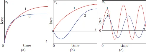
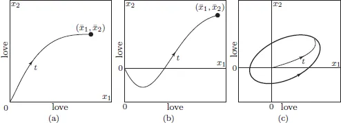
Table of contents

• Cover
• Halftitle
• Series Editors
• Title
• Copyright
• Contents
• Preface
• 1. Can we model love stories?
• Simple models
• Complex models
• Appendix A Appendix
• Bibliography
• Index