![]()
Chapter 1
Introduction
1.1Background
During the past four decades, huge efforts have been dedicated to manage data that is deterministic, and the successful deployment of commercial DBMSs deeply influences human life. Most recently, it becomes critical to process uncertain (probabilistic) data, since data uncertainty widely exists in many applications, such as economy, military, logistic, finance, and telecommunication, etc. The causes for uncertain data include, but are not limited to the following: low-end physical equipments, manual intervention, data missing, and data integration [82].
- Low-end physical equipments. Data may be imprecise due to low-end physical equipments, such as sensor networks [29]. Data accuracy is also affected by bandwidth, transmission delay and energy during wireless network transmission process. It is reported that more than 30% of tag readings in the RFID applications are dropped [46].
- Manual intervention. Manual intervention helps to achieve special targets, such as privacy preserving. For example, modern GPS-enabled electronic devices can track the trajectories of moving objects, such as intelligent mobile phones. A common way to protect location privacy (called k-anonymity) uses an area to describe the actual location of a user, so that he (she) cannot be distinguished from the other k − 1 users.
- Data missing. Data missing occurs in many cases, including equipment failure, invalid access, data inconsistent, and historical usage. Although some existing data cleaning mechanisms can eliminate uncertainty by assuming the underlying data follows a distribution or simply ignoring incomplete records, they cannot describe the nature of data uncertainty well.
- Data integration. Data integration also brings in uncertainty, since the data from different sources may be inconsistent. By integrating multiple sources of uncertain data, it is helpful to resolve portions of the uncertainty to achieve more accurate results [7].
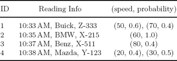
A significant trend in the modern applications is that the uncertain data tends to be gathered in a streaming fashion. For example, each sensor node in a senor network gathers and transfers data to a main site continuously; RFID tags are read continuously. Table 1.1 illustrates a small example of modern traffic monitoring applications, where radars are used to detect the speed of vehicles. There are four tuples, each described as a discrete probability distribution function rather than a single value, since some errors may be caused for complicated reasons, such as nearby high voltage lines, close cars’ interference, human operator mistakes, etc. For instance, the 1st record observes a Buick car (No. Z-333) running through the monitoring area at 10:33AM with the speed estimated as 50 (miles per hour) with probability 0.6, and 70 with probability 0.4 respectively. In addition, a range is used to test the validation of a speed reading (e.g., [0, 120]). Once the reading exceeds the range, this information is removed from the tuple description, which makes the total confidence smaller than 1. For example, the 3rd record estimates the speed of 80 with probability 0.4, and of invalidation with probability 0.6 (= 1 − 0.4).
Table 1.1 A Radar Reading Data Stream
There are two kinds of uncertainties: attribute-level uncertainty and existential uncertainty. The latter is also called as tuple-level uncertainty in some literatures [2]. The attribute-level uncertainty, commonly described as discrete probability distribution function or probability density function, illustrates the imprecision of a tuple’s attributes, e.g., the first tuple. The existential uncertainty describes the confidence of a tuple, e.g., the third tuple. A tuple may have two kinds of uncertainties at the same time, such as the last tuple.
Uncertain data streams have attracted a lot of attention [5, 20, 44, 45, 78]. Since large amounts of such streaming data arrive rapidly, the goal is to design both space- and time-efficient query processing techniques, which only require to visit each tuple once. On the other hand, streaming data is also highly time-sensitive: people are generally more interested in the recent tuples than those in the far past, which further adds the challenges of uncertain stream processing.
1.2Data Model
The model for uncertain data streams is actually the integration of data uncertainty and streaming property. Most uncertain data models adopt the possible world semantics [1, 36], in which the possible world space contains a huge number of possible world instances (also shorten as possible world), each consisting of a set of certain values from uncertain tuples. A possible world instance is affiliated with a probability value, computed by the product of all tuples within the instance and the product of the non-existing confidence of all tuples outside.
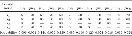
Table 1.2 illustrates the possible world space of total 12 instances for the data stream in Table 1.1. Each column is a possible world instance with the probability listed below. For example, tuples t1, t2 and t3 occur in pw10 at the same time, while t4 does not occur, so the probability of pw10 is computed as 0.016 (= 0.4 × 1.0 × 0.4 × (1 − 0.4 − 0.5)).
Table 1.2 The Possible World Space for Table 1.1
In general, an uncertain stream
S is defined as
S = {
t1,
t2, . . .}, where an uncertain tuple
ti appears at timestamp
i. Each tuple is described as a discrete probability distribution function,
ti = 〈(
vi,1,
pi,1,), . . . ,(
vi,mi,
pi,mi)〉, meaning that
ti can be one of
mi different certain values, denoted as
vi,1, . . . ,
vi,mi, with confidence of
pi,1, . . . ,
pi,mi. The sum of the probabilities of all choices is no greater than 1, i.e.,
. Especially, if only existential uncertainty exists, ∀
i ≥ 1,
mi = 1 [
20].
The streaming models can be categorized into the landmark, time-decay, and sliding-window models according to time aspect. The landmark model considers all tuples from a fixed time point to now. The time-decay model assigns a weight to each tuple, and the weight will decrease over time. This model usually works together with statistical aggregates, such as averages, histograms, and heavy hitters [21, 24]. The sliding-window model only considers all tuples within a pre-defined window W. In other words, the rest ones outside the window are filtered. For example, assuming W = 5, the window is [6, 10] at time 10.
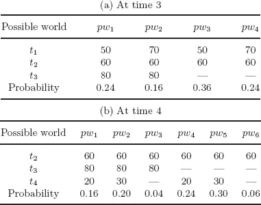
One major challenge of uncertain data management is that the possible world space will grow up exponentially to the size of the uncertain database. Suppose there are N independent tuples in an uncertain database, the number of the possible world instances is O(2N). Hence, it is infeasible to access all possible world instances one by one even when N is not tiny. Therefore, it is necessary to make a trade-off between the accuracy and overhead, so as to obtain high-quality approximate results with small computational overhead. Moreover, the possible world space will change a lot when a new tuple arrives, no matter upon the landmark model or the sliding-window model. For example, assuming W = 3, Tables 1.3(a) and 1.3(b) show the possible world space for the data in Table 1.1 at times 3 and 4 respectively. We observe that all possible world instances change.
Table 1.3 The Possible World Space for Table 1.1 over the Sliding-window Model (W = 3)
Furthermore, we also study a more comprehensive model in Chapter 5 where each tuple in the data stream is no longer a single value, but a set of probabilistic tuples. An example data stream may be: {{1:0.7, 2, 1.0}, {2:0.5, 3:0.7, 4:0.4}, . . .}. In this stream, the first set, {1:0.7, 2,1.0}, contains two tuples, 1 and 2, each with probability 0.7 and 1.0. The second set in the data stream contains three tuples, and so on. Similarly, we can construct a joint-possible world space based on any of two probabilistic sets.
For example, consider two probabilistic sets A and B in Table 1.4. They have eight (joint) possible worlds, which are listed together with their similarities and existential probabilities in Table 1.4(b). For example, the ...