Cosmology with MATLAB

With Companion Media Pack

Dan Green

• Publisher: WSPC
• Year: 2016
• ISBN:
  9789813108424
• Topic: Naturwissenschaften
• Subtopic: Astronomie & Astrophysik

This volume makes explicit use of the synergy between cosmology and high energy physics, for example, supersymmetry and dark matter, or nucleosynthesis and the baryon-to-photon ratio. In particular the exciting possible connection between the recently discovered Higgs scalar and the scalar field responsible for inflation is explored.

The recent great advances in the accuracy of the basic cosmological parameters is exploited in that no free scale parameters such as h appear, rather the basic calculations are done numerically using all sources of energy density simultaneously. Scripts are provided that allow the reader to calculate exact results for the basic parameters. Throughout MATLAB tools such as symbolic math, numerical solutions, plots and "movies" of the dynamical evolution of systems are used. The GUI package is also shown as an example of the real time manipulation of parameters which is available to the reader.

All the MATLAB scripts are made available to the reader to explore examples of the uses of the suite of tools which are available. Indeed, readers should be able to engage in a command line "dialogue" or go on to edit the scripts and write their own versions.

Contents:

• Introduction
• From the Big Bang
• Inflation and Big Bang Issues
• Fluctuations to Perturbations
• The Cosmic Microwave Background
• Large Scale Structure
• The Higgs Boson and Inflation
• Appendices:
  • MATLAB Tools
  • Power Law, RD or MD Formulae
  • Symbol and Acronym Tables
  • MATLAB Script (with Companion Media Pack)

Readership: Graduate students and researchers in physics.

Chapter 1

Introduction

“Mathematics expresses values that reflect the cosmos, including orderliness, balance, harmony, logic, and abstract beauty.”

— Deepak Chopra

“When you look at the stars your eyes are time machines.”

— Waqas Rabbari

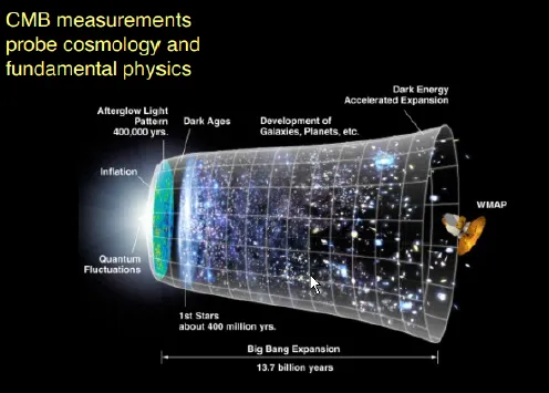
There are several basic parameters in the SM of cosmology. This section makes a self-contained exposition of the basic facts of big bang (BB) cosmology as they relate to inflation. The SM appears schematically in Figure 1.1. Inflation starts the Universe on a path of rapidly growing size. After inflation the Universe evolves more sedately to the time of CMB creation when photons decouple from matter and then almost freely propagate to us some 14 billion years later. After the “dark ages” stars form and over time matter aggregates, since gravity is always attractive and wins in the long run. Large scale structures (LSS) develop with time. Finally, dark energy (DE) begins to dominate over matter and radiation and the size of the Universe again begins to increase rapidly.

The CMB is the cooled fireball of the Big Bang. Photons at the present CMB temperature have wavelengths ∼0.2 mm. The CMB is known to have a uniform temperature to parts per 10⁵ but has [5], [6] well-measured temperature perturbations and the associated baryon, proton, perturbations are thought to evolve gravitationally and thus to provide the seeds of the current structure of the Universe.

In addition, the Universe appears to contain, at present an unknown “dark energy” [7] which is currently the majority energy density of the Universe, larger than either matter or radiation. This may, indeed, be a fundamental scalar field like the Higgs with a vacuum expectation value which defines a cosmological constant or it may evolve in time as a dynamical field. At present DE is compatible with a constant vacuum energy density and it will be assumed to be such in what follows.

Figure 1.1: Artist’s conception of the complete history of the Universe.

“Big Bang” cosmology is a very successful “standard model” (SM) in cosmology [8]. The CMB is the cooled remnant of the BB. The abundances of the light nuclei from an early hot phase are accurately predicted by BB cosmology. However, the model cannot explain the uniformity of the CMB because the CMB consists of many regions not causally connected in the context of the BB model. In addition, the Universe appears to be spatially flat [9]. However in BB cosmology the spatial curvature is not stable and grows with time so that the initial conditions for BB cosmology would need to be fantastically fine-tuned in order to successfully predict the presently observed small value, consistent with zero, of the curvature of space-time.

These basic issues for BB cosmology have led to the hypothesis of “inflation” which postulates an unknown scalar field which causes an exponential expansion of the Universe at very early times [10], [11]. This attractive hypothesis can solve the problems of flatness and causal CMB connectivity which are inherent in BB cosmology. The homogeneity and isotropy of the observable Universe are also simply explained. In addition, the zero point quantum fluctuations of this postulated field provide a natural explanation of the CMB temperature perturbations and the associated LSS of the Universe. Researchers are now searching for gravitational waves imprinted on the CMB [12], [13]. If detected they would be strong evidence for inflation since metrical fluctuations are produced in inflationary models.

This text makes a very basic exposition of the BB cosmology and an inflationary model using MATLAB tools for visualization and in order to build up an intuition on the parametric dependence of the observables. The simple scalar model, with a potential proportional to the square of the field, is explored in detail first because it is easy to understand, contains all the basic elements of the inflationary model [12], and is presently consistent with the data. Another model with a potential proportional to the fourth power of the field is covered briefly for comparison.

Finally, the Higgs field could be the inflationary field, although a non-minimal coupling of the Higgs to gravity is needed. Nevertheless, this is an economical model requiring no new fields to be invoked although there are issues of the stability of the vacuum if no new physics intervenes between the Higgs mass of 126 GeV and the Planck mass of 1.2 × 10¹⁹ GeV, an immense energy range. This range is not accessible to laboratory experimentation so that cosmology is, at present, the sole method of exploring these energies, although precise laboratory experimentation might be sensitive to very small effects caused by these very high energy phenomena.

Using the methods shown in the text to compare these three models of inflation to the present data allows the user to explore any other specific model. The reader will be able to compute the observables for any model of inflation and assess the viability of that particular model as the data improves with time.

1.1.Cosmic Numerology

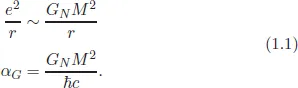
The units used in the text are GeV, m, and sec. There is only one coupling constant, the gravitational constant of Newton, G_N, which has dimensions in contrast with the dimensionless couplings of particle physics (Eq. (1.1)). That points to the fact that gravity is not a renormalizable theory. Because of that, there is presently no quantum theory of gravity with interacting point particles and by default classical general relativity (GR) will be assumed. That means very high energies and very small distances cannot strictly be covered in GR. A quantum theory of gravity remains a major problem in physics one hundred years after the advent of GR.

The gravitational coupling constant, α_G, is subsumed by using the Planck mass to set mass scales. Since inflation deals with very high energies, the Planck mass, M_p, is a natural scale, one where the gravitational coupling constant becomes of order unity. Related scales are the Planck length L_p and the Planck time t_p (Eq. (1.2)). Natural units are used in the text, = c = 1, G_N = 1/M²_p, so that, in principle, all quantities could be expressed in energy units. The Boltzmann constant is also set equal to one so that temperature is in energy units. Some papers use G_N = 1 units which can be confusing, but M_p is always explicitly used here. In addition some papers use a reduced Planck mass which differs by a factor √8π from this definition and should be watched for.

For explicit numerical values the MATLAB script supplied here should be examined because the scripts are used to convert to physical units such as GeV, m and sec. For energies of order ...

Table of contents

• Cover
• Halftitle
• Series Editors
• Title
• Copyright
• Preface
• Contents
• 1. Introduction
• 2. From the Big Bang
• 3. Inflation and Big Bang Issues
• 4. Fluctuations to Perturbations
• 5. The Cosmic Microwave Background
• 6. Large Scale Structure
• 7. The Higgs Boson and Inflation
• Appendix A: Matlab Tools
• Appendix B: Power Law, RD or MD Formulae
• Appendix C: Symbol and Acronym Tables
• Appendix D: MATLAB Script (with Companion Media Pack)
• References
• Index