Elements of Stochastic Dynamics

Guo-Qiang Cai, Wei-Qiu Zhu

• Publisher: WSPC
• Year: 2016
• ISBN:
  9789814723343
• Topic: Technology & Engineering
• Subtopic: Mechanical Engineering
• Index: Technology & Engineering

Stochastic dynamics has been a subject of interest since the early 20th Century. Since then, much progress has been made in this field of study, and many modern applications for it have been found in fields such as physics, chemistry, biology, ecology,

CHAPTER 1

INTRODUCTION

Modeling and analysis of dynamical systems are a critical task in almost all areas, such as physics, chemistry, biology, meteorology, ecology, economy, finance, and many branches of engineering including mechanical, ocean, civil, bio and earthquake engineering. In the modeling process, uncertainties are present inevitably due to various factors, such as possible changes of system parameters, variations in excitations, errors in modeling schemes, etc. To take into consideration of the uncertainties more accurately, observations and measurements are usually carried out to obtain data as much as possible. If the amount of the data for a specific uncertainty is large enough, this uncertainty can be described by means of probability and statistics. Specifically, if the uncertain physical quantity is a time-independent variable, it can be represented by a random variable. On the other hand, if the physical quantity is a time-varying process, it can be modeled as a stochastic process.

The earliest investigation of stochastic dynamics was due to Einstein in 1905 (Einstein, 1956), who developed a stochastic model for Brownian motion, a type of chaotic motion of small particles floating on water. The term of “Random Vibration”, widely used in civil and mechanical engineering, was first proposed by Rayleigh (1919) for an acoustic problem. Study of random vibration began in the 50’s in three aeronautical problems: buffeting of aircrafts due to atmosphere turbulence, acoustic fatigue of aircrafts caused by jet noise and reliability of payloads in rocket-propelled space vehicles. The common factor in the three problems was the random nature of the excitations. Since then, investigation of systems under random excitations has been promoted to solve problems in aeronautical and astronautical, mechanical and civil engineering. The systems have been extended for linear to nonlinear, and the excitations from external to parametric. A survey of the development in the field of random vibration in the first three decades was given by Crandall and Zhu (1983). With rapid advancement of computer technology, more practical problems in various areas with many degrees of freedom and strong nonlinearity can be solved numerically using simulation techniques.

It is noticed that the term of random vibration has been used widely when responses and reliabilities of stochastic systems are of concern. Thus, development of solution methods is the main objective. If, besides the responses and reliabilities, the qualitative behaviors of stochastic systems, such as stability and bifurcation, are also the objectives of the investigation, the term “Stochastic Dynamics” is usually used, and it covers more topics than those in random vibration.

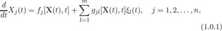
A stochastic dynamical system may be described by the following stochastic differential equations

where X(t) = [X₁(t), X₂(t), . . . , X_n(t)]^T is a vector of system response, also known as state variables, the superscript T is a notation for matrix transposition, ξ_l(t) are excitations and at least one of them is stochastic process. Note that the capital letters used in (1.0.1) for the state variables signify that they are random or stochastic quantities. Functions f_j and g_jl represent system properties which may or may not depend on time explicitly. An excitation ξ_l(t) is called a parametric (or multiplicative) one if the associated function g_jl depends on X; otherwise, it is known as an external (additive) excitation.

If all functions f_j are linear functions of X and functions g_jl are all constants, the system is linear. If all functions f_j and g_jl are linear functions of X, it is known as parametrically excited linear system, although it is essentially nonlinear since the superposition principle is no longer applicable. If at least one of the functions f_j and g_jl is nonlinear, it is a nonlinear system. For the case of n = 1, it is a one-dimensional system. Otherwise, it is called a multi-dimensional system. A continuous system governed by a partial differential equation can be discretized to a multi-dimensional system using schemes such as finite-element procedure.

The stochasticity (randomness) may occur in system properties, in which case some parameters in functions f_j and g_jl are random variables. It may occur in excitations, namely, some of excitations ξ_l(t) in Eq. (1.0.1) are stochastic processes. In this book, only the latter case is considered, and systems properties represented by functions f_j and g_jl are assumed to be deterministic.

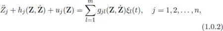
Equations of motion of many mechanical and structural systems are usually established by means of the Newton’s second law or the Lagrange equations according to the physical nature. The governing equations often appear in the following form

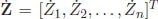
where Z = [Z₁, Z₂, . . . , Z_n]^T and

are vectors of displacements and velocities, respectively, and h_j(Z,

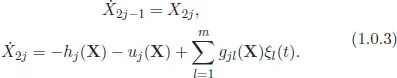
) and u_j(Z) represent damping forces and restoring forces, respectively. Letting X_2j−1 = Z_j, X_2j =

_j and X = [X₁, X₂, . . . , X_2n]^T, system (1.0.2) is transformed to

By comparison of (1.0.3) and (1.0.1), it can be seen that equation set (1.0.3), is a special case of system (1.0.1). Conventionally, system (1.0.2) is known as an n-degree-of-freedom system, which is equivalent to a 2n-dimensional system (1.0.1). These two technical terms will be followed throughout this book, namely, the term of “degree-of-freedom” is used for second-order system, while the term “dimension” is used for first-order systems. For example, a singledegree-of-freedom system is a two-dimensional system, and an n degrees-of-freedom system is a 2n-dimensional system.

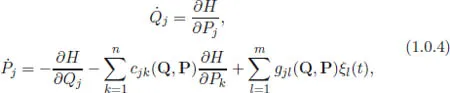
A stochastic dynamical systems can also be formulated as stochastically excited and dissipated Hamiltonian system, governed by the equations

where Q_j and P_j are generalized displacements and momenta, respectively, Q = [Q₁, Q₂, . . . , Q_n]^T, P = [P₁, P₂, . . . , P_n]^T and H = H(Q, P) is a Hamiltonian function. Equation set (1.0.2) can be transformed to the form of (1.0.4) by using the Legendre transform. It can be seen that the stochastically excited and dissipated Hamiltonian system (1.0.4) is also a special case of system (1.0.1).

Mathematically, equations of motion of (1.0.1) are more general than (1.0.2) and (1.0.4) since the latter two equation sets can be transformed to the former equation set. However, for many engineering systems, Eqs. (1.0.2) are usually derived directly from Lagrange equations, and then transformed to (1.0.4). They describe the relationships between different degrees of freedom. The methods and procedures introduced in the book, although applicable to the general system (1.0.1), are especially suitable for systems (1.0.2) and (1.0.4).

The vectors X(t) = [X₁(t), X₂(t), . . . , X_n(t)]^T in system (1.0.1), Z = [Z₁, Z₂, . . . , Z_n]^T and

= [

₁,

₂, . . . ,

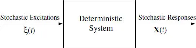
_n]^T in system (1.0.2), Q = [Q₁, Q₂, . . . , Q_n]^T and P = [P₁, P₂, . . . , P_n]^T in system (1.0.4) are known as system responses. Moreover, their functions, such as the system Hamiltonian, the amplitude envelope of a single response, and the system total energy, also belong to the category of system responses. Although the systems considered in this book are deterministic, the system responses are stochastic processes due to the stochastic excitations, as illustrated in Fig. 1.0.1.

Figure 1.0.1 System excitations and responses.

With system models established deterministically, the most important element is the stochastic excitations, which must be modeled properly based on their characteristics in the involved physical problems. A large amount of data must be acquired from tests, experiments or real-time measurements in order to model a real physical excitation as a stochastic process described by statistical and/or probabilistic characteristics. Among the statistical characteristics, the mean value, mean square or variance, correlation function or spectral density are the most important. The probability distribution may be also important in certain practical problems (Wu and Cai, 2004). If the probability distribution can be inferred from available data, the mean and mean square can be calculated. In general, the power spectral density and probability density are the most desirable to model a stochastic process.

The classification of stochastic processes depends on the criterion chosen. According to their probability distributions, stochastic processes may be called Gaussian processes, Rayleigh processes, Poisson processes, bounded processes, etc. The Gaussian distribution is very popular due to several reasons: (a) the bell-shape of the Gaussian probability density indeed matches the shapes of many practical probability densities, (b) it can be defined completely only by two parameters, the mean and mean square and (c) its mathematical treatment is simple. One of the drawback of the Gaussian distribution is the unbound nature of the process even with a small probability. To overcome it, models of different types of bounded processes are described in the book. If the criterion is the frequency bandwidth of the spectral density, stochastic processes can be classified as narrowband processes and broad-band processes. A harmonic process is a limiting case of narrow-band process with an infinitely narrow band. On the other hand, the widely used so-called white noise is a limiting case of broad-band process with a constant spectral density over an infinite bandwidth. Although it is an ideation of real broad-band processes, it has been used in many problems since it is easy to treat mathematically and system responses decay very rapidly in the range of higher frequency. Another criterion to classify stochastic processes is their time-evolutionary nature. Conceptually, a process is stationary if its probability density and spectral density do not change with time; otherwise, it is a non-stationary process (accurate definitions of stationarity are given in Chapter 3). Many real excitations lasting for long time duration, such as ocean wave forces, wind forces, forces to vehicles from road roughness, etc., may be considered as stationary processes in...

Table of contents

• Cover
• Halftitle
• Title
• Copyright
• Preface
• Contents
• About the Author
• Chapter 1 Introduction
• Chapter 2 Random Variables
• Chapter 3 Stochastic Processes
• Chapter 4 Markov and Related Stochastic Processes
• Chapter 5 Responses of Linear Systems to Stochastic Excitations
• Chapter 6 Exact Stationary Solutions of Nonlinear Stochastic Systems
• Chapter 7 Approximate Solutions of Nonlinear Stochastic Systems
• Chapter 8 Stability and Bifurcation of Stochastically Excited Systems
• Chapter 9 First-Passage Problem of Stochastically Excited Systems
• References
• Index