Deep Dive into Financial Models

Modeling Risk and Uncertainty

Mathieu Le Bellac, Arnaud Viricel

• Publisher: WSPC
• Year: 2016
• ISBN:
  9789813142121
• Topic: Business
• Subtopic: Financial Risk Management
• Index: Business

-->

Since 2007, the repeated financial crises around the world have brought to the headlines financial practices and models considered to fuel the economic instabilities. Deep Dive into Financial Models: Modeling Risk and Uncertainty comes handy in demystifying the underlying quantitative finance concepts. With a limited use of mathematical formalism, the book explains thoroughly the models, their hypotheses, principles and other building blocks. A particular care is given to model limitations and their misuse for investment strategies, asset pricing, or risk management. Its reader-friendly nature provides readers with a head start in quantitative finance.

-->

Request Inspection Copy

--> Contents: Interest Rate Curve;Principal Component Analysis;Risk Free Rate;Credit Spread;Merton Model;Credit Correlation;Markowitz Theory;Capital Asset Pricing Model;Cointegration;No Arbitrage Theory;Black Scholes Model;Implied Volatility;Volatility Surface;Volatility Models;Dupire Model;Heston Model;Monte Carlo Methods;Finite Differences Methods;Value at Risk;Fat Tail Models;Levy Processes;
Readership: Undergraduate and graduate students who are taking up Quantitative Finance courses and those who possess college mathematical background.
Quantitative Finance, Mathematical Finance, Applied Mathematics to Financial Markets, Arbitrage, Quantitative Analysis, Financial Engineering, Valuation Model, Derivative Pricing, Financial Model Review

• More emphasis on the founding principles and the consequences of financial models which provides a thorough understanding on the subject
• Numerous reader-friendly and original graphs which help gain an intuitive view on the physical properties of financial concepts
• A critical look on the models as assessed by professional risk managers

Chapter 1

Interest Rates

Benjamin Franklin stated “Time is money”. This applies in particular to the financial world, where it is materialized by interest rates. It seems indeed natural that all loaned money must have some payment as a counterpart: we shall consider that the payment of interests is aimed at compensating the loss, by the lender, of other profitable investment opportunities or of consumption capacities. Interest rates also take into account the risk that the loaned sum is not reimbursed. This risk is called the credit risk and it will be addressed in the next chapter.

In the present chapter, we shall introduce the notions of interest rates and of present valuation (section 1) and we shall demonstrate the existence of a term structure of interest rates (section 2). We shall finally study in section 3 the time evolution of the interest rates curve by relying in particular on the Principal Component Analysis introduced by [Litterman and Scheinkman 1991].

1.1Present valuation

The purpose of interests is to pay the lender, or the creditor, for having made available some amount of money to the borrower, during a time period and according to specific terms of payment. The range of available options is quite large: the duration of the loan, generally called the maturity, may vary from 24 hours to half a century; the capital may be reimbursed progressively, as in a retail real estate loan, or fully at maturity. Whatever the type of loan, the borrower must be able to compute an interest rate in order to assess the cost of the loan and to compare the different configurations which may be offered.

When we put money on a savings account, we lend money to our bank and we are entitled to a payment as a counterpart. Thus, $100 invested at a yearly interest rate of 2% capitalize and become $102 at the end of the year. If the sum is fully reinvested into a savings account under the same conditions, after a second year of bearing interest, it will be worth 102 × (1 + 2%) = $104.04, then $100 × (1 + 2%)³ in the third year, . . . , and $100 × (1 + 2%)ⁿ in the n^th year. This calculation shows that after 10 years, we own about $122: the 2% interest rates have brought us more than 10 times the yearly interest rate, as all the interests have been reinvested and have capitalized in turn. This is the convention on which all our calculations will be grounded: the interests unpaid to the lender at the end of the period during which the rate is applied generate further interests at the same rate.

With this convention, an amount M which capitalizes at the yearly interest rate r will be worth M × (1 + r)^T after T years. Thus, theory implies that, had Platon invested $1 in 400 BC at a 1% yearly rate, he would own $(1.01)²⁴¹⁶ today in 2016, namely more than $25 billion.

Let us reverse our viewpoint and assume that we would like to own $100 in 10 years: what amount of money should we invest? The calculation is very simple: the answer is $100/(1 + r)¹⁰, which is about $82 given an interest rate r = 2%. This property may be conceptualized the following way:

It is equivalent to own $82 today or to own $100 in 10 years.

What we must pay today to own $100 in 10 years is $82.

The present value of $100 in 10 years is $82 today.

We have just introduced the fundamental notion of discounted value, also called the present value. This value is simply the price to be paid today in order to receive a future cash flow. In our example, the present value of $100 to be collected in 10 years is $82. When one uses an interest rate to compute the present value of a payment, then this rate is called the discount rate. A large part of financial mathematics which we are going to uncover in the following chapters addresses the calculation of the present value of future cash flows, known or unknown. This value is today’s market price of those future cash flows, that is, the price at which traders are ready to buy or to sell these cash flows.

Box 1.1. Present valuation, or discounting. Discounting is the computation of today’s value of a future cash flow. This computation depends on the level of interest rates: if the yearly interest rate is 5%, the present value of a $105 cash flow to be collected in one year is $100. Therefore, present valuation allows one to compare the value of cash flows paid at different dates.

Let us summarize where we stand using a slightly more sophisticated example. Assume you are the representative of a Government and you wish to borrow on financial markets. You are ready to pay $5 M for the first two years and reimburse $105 M at the end of those 3 years. Given a 2% discount rate, how much will you be lent? In other words, what is the present value of the cash flows? The answer is readily computed:

Indeed, each cash flow to be collected has a price: the first one is worth 5/(1 + 2%) ≃ $4.9 M, the second one 5/(1 + 2%)² ≃ $4.8M and the last one 105/(1+ 2%)³ ≃ $98.95 M. The total cost is the sum of the prices of each cash flow.

It is very important to be able to compute at any time this present value of the cash flows which the Government pays, as the loan granted may be resold by the lender on financial markets to another market participant wishing to own a Government debt. In order to do so, the Government loan often takes the form of a bond. A bond operates exactly as a loan whose advantage is that it can easily be exchanged on financial markets: it is the holder of the bond who collects the reimbursement flows from the borrower who issued the bond. A whole jargon was developed around these bonds: the amount of capital is called the face value of the bond and the interests which are paid, the coupons. In general, the coupons are known in advance and fixed as a percentage of the face value of the bond: one then speaks of fixed rate bond. The face value of the bond is then reimbursed together with the last coupon at maturity.

Box 1.2. Bonds. A bond is a security, that is an asset tradable on financial markets, which represents the debt of a Government or of a company towards the holder of the bond. Thus, the owner of the bond, the bondholder, is the creditor of the debt. He is entitled to receive at fixed intervals of time some amount of interests called a coupon, computed as a percentage of the capital (also named the face value, or the nominal) which the borrower must reimburse at maturity.

In the example of equation (1.1), we computed the present value, that is, the price of a bond reaching its maturity in 3 years, whose face value is $100 M and with yearly coupons of 5%. If the interest rates are 2%, an investor will therefore buy the bond at a price of $108.65 M.

Our presentation may puzzle the reader who attempts to link bonds with retail real estate loans. In our example:

The amount paid by the investor to buy the bond, $108.65 M, is not the face value, which is $100 M.

The coupon rate, 5%, which is the interest paid to the bondholder, is different from the interest rate used for discounting, which is 2%.

In our presentation of the bonds, the face value is reimbursed at the end of the loan only, in other words, it is not amortized over the lifetime of the loan.

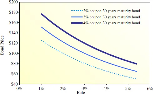
If the interest rates matched exactly the coupon rate, 5%, the price of the bond would match the face value of $100 M. However, in practice, interest rates vary constantly on the markets (similarly to the rate of a savings account which varies during the year). Let us assume that the sovereign bond was issued at a time when the interest rate was 5%. In our example, the interest rate then went down to 2%. The sovereign bond brings now more interests than the market’s interest rate: it is logical that its price has risen and that it is worth more than its face value. The fall in interest rate has therefore increased the price of the bond. Conversely, it seems clear that the right to receive fixed interests is less interesting when the rates increase and market participants have the opportunity to invest into products which take this rise into account. This explains the famous rule according to which the price of bonds falls when interest rates rise, and conversely (Figure 1.1).

Figure 1.1: Variation of bond prices as a function of the interest rate. One must notice that (i) for the same rate and the same maturity, the bond prices rise with the value of the coupons; (ii) the bond prices decrease with the level of the interest rates; (iii) the curves giving the bond prices are not straight lines and they are steeper as the interest rates decrease.

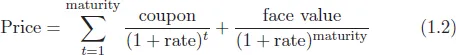
More formally, the equation which links the discount rate, the price, the coupons, the maturity and the face value of a bond is:

If all parameters of this equation but the discount rate are fixed, then there is only one rate which satisfies equation (1.2). This rate is called the yield of the bond. From the very way the equation is built, the yield represents the true return of the bond, since it is strictly equivalent to buying the bond ...

Table of contents

• Cover Page
• Title
• Copyright
• Contents
• Preface
• Foreword
• 1 Interest Rates
• 2 Credit Risk Modeling
• 3 Portfolio Management Theories
• 4 No-arbitrage Theory
• 5 The Black-Scholes Model
• 6 Volatility Models
• 7 Numerical Methods
• 8 Value at Risk (VaR)
• 9 Non-Gaussian Models
• Conclusion
• Bibliography
• Index