International Economics

Global Markets and Competition

Henry Thompson

• Publisher: WSPC
• Year: 2017
• ISBN:
  9789814663892
• Edition: 4
• Topic: Economics
• Subtopic: Macroeconomics
• Index: Economics

-->

International Economics: Global Markets and Competition integrates the microeconomics of international trade with open economy macroeconomics and finance. The theory is comprehensive but presented with intuitive diagrams. The book emphasizes the gains from international competition and the limits of trade policy.

Economics began during the Industrial Revolution with a debate over import tariffs. To this day, domestic industries lobby for tariff protection against foreign competition, paying lawmakers for tariffs on imports. Only under special conditions do tariffs lead to economic gains. Domestic importers of materials and industrial products favor free trade, as do export industries since tariffs encourage other countries to retaliate with tariffs of their own.

Trade theory includes market analysis and general equilibrium models of the economy. This text integrates the full range of trade theory with exchange rates, balance of payments, international finance, and open economy growth and macroeconomics.

The presentation focuses on diagrams and avoids equations and algebra. The theory is presented with numerical examples. The text does not assume intermediate economics, instead developing the theory with thorough explanations. Questions in each section build confidence in applying the theory. Boxed examples illustrate the importance of the theory.

Students like the concise and straightforward style. Instructors notice the difference on exams.

-->

Request Inspection Copy

-->

INTERNATIONAL MACROECONOMICS

CHAPTER 10

Balance of Payments

Preview

This chapter introduces the balance of payments BOP. Issues range from how to finance a trade deficit to what happens to the foreign currency of a trade surplus. A related issue is the effect of a government deficit on the BOP. The potential of government policy to influence the BOP is examined. This chapter examines:

•Import and export elasticities and the trade balance

•Components of the BOP

•The government budget and the BOP

•International roles of fiscal and monetary policies

INTRODUCTION

If the price of an import rises, import quantity falls. If imports fall enough, import spending falls even with the higher price. The imports of one country are the exports of another implying the balance of trade depends on how sensitive imports are to changing prices.

For economies dependent on trade, international price changes can be critical. For instance, changes in the price of oil cause adjustments for both exporters and importers.

Countries may not spend on imports what they earn from exports during a year. The current account in the balance of payments BOP includes trade in goods and services plus net interest payments. If the current account is not zero, there is international borrowing or lending in the capital account. This chapter describes the fundamental mechanisms of BOP adjustment in the current and capital accounts.

Government economic policy may influence the BOP. Fiscal policy refers to government spending and taxes. Monetary policy refers to government control of the money supply. This chapter examines now fiscal and monetary policies influence the BOP.

A. ELASTICITIES AND THE TRADE BALANCE

Changing prices of traded goods affect export revenue and import spending. Changing prices of merchandise imports and exports affect the balance of trade BOT equal to export revenue minus import spending. The balance on goods and services BGS includes trade in services,

Changing Export Prices and the BGS

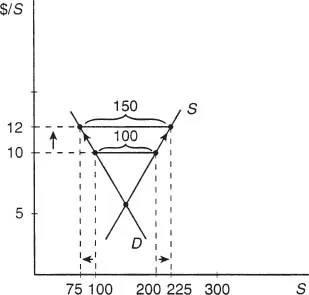
A higher export price increases production and export revenue but domestic consumers pay the higher price. In Figure 10.1 at a world price of $10, exports equal 100 units of services. Production is 200 units and 100 units are consumed. Exporters can sell as much as they want at the international price. If price rises to $12 domestic consumers cut consumption to 75 and producers increase output to 225. Excess supply or exports expand to 150.

Selling more services at the higher price increases export revenue. The level of exports rises by 50, export revenue rises from $1000 to $1800, and total revenue of domestic firms rises from $2000 to $2700. Domestic consumers pay a higher price and consume less. Consumers spend $900 on 75 units, less than the previous $1000 on 100 units.

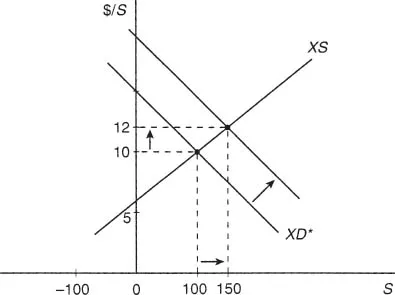
A higher export price is illustrated with the increase in foreign excess demand in Figure 10.2 consistent with Figures 10.1. The higher foreign excess demand in Figure 10.2 is the cause of the higher price in Figure 10.1. In Figure 10.2 the price increase is endogenous, explained by the model. In Figure 10.1, the price change is exogenous, outside the model.

Figure 10.1
Increased Export Prices
When the price of exported services rises from $10 to $12 exports rise from 100 to 150. Producer surplus rises but consumer surplus falls.

Figure 10.2
Increased Foreign Excess Demand
An increase in foreign excess demand XD^* raises the international price from $10 to $12 and raises the quantity exported from 100 to 150.

Increased export prices raise export revenue and the BGS.

EXAMPLE 10.1 Price Taking Small Open Economies

Are small economy exporters price takers? Arvind Panagariya, Shekhar Shah, and Deepak Mishra (2001) find that Bangladesh faces an import elasticity of 26 in textiles and apparel products. A 1% increase in the price of these products by Bangladesh reduces the quantity of exports by 26%, very elastic. These exporters in Bangladesh have no market power, making the price taking assumption reasonable.

Import Prices and the BGS

Imports are inversely related to price. An increase in the price of an import lowers quantity demanded and raises the quantity supplied.

Examples of increased import prices include the Organization of Petroleum Exporting Countries (OPEC) tripling the price of oil in the 1970s, bad weather in Colombia driving up the international coffee price, and dollar depreciation raising the price of imported cars from Germany.

Consider the exogenous increase in the price of imported manufactures from $5 to $7.50 in Figure 10.3. Domestic quantity demanded falls from 300 to 250. Spending by domestic consumers increases from $1500 to $1875. The quantity supplied domestically rises from 100 to 150. Revenue of domestic firms rises from $500 to $1125.

Figure 10.3
Higher Import Prices
An increase in the price of imports from $5 to $7.50 increases quantity supplied from 100 to 150. Domestic quantity demanded falls from 300 to 250. Imports fall from 200 to 100. Import spending falls due to the elastic imports.

Import spending falls from $1000 to $750, raising the BGS. Import spending may rise, however, depending on the import elasticity.

Import Elasticity

If there is little opportunity for adjustment to a higher import price, import demand is inelastic. A price increase then results in increased import spending.

If the price of imports and import spending are negatively related as in Figure 10.3 import demand is elastic. If consumers and firms adjust imports, import spending falls.

In the 1970s at the time of increased oil prices, consumers were driving large inefficient cars. Oil imports were inelastic and OPEC oil export revenue rose.

In the face of consistently high oil prices, cars became more fuel efficient. Houses were insulated and heating and cooling technology improved. Oil consumption fell. The quantity of oil supplied domestically increased. OPEC learned about import elasticity as their export revenue tapered and imports proved more elastic.

The import elasticity summarizes the relationship between import prices and spending,

The symbol Δ means “change in” and %ΔX is “the percentage change in X”. Quantity Q_imp and price P_imp are inversely related.

To find percentage changes subtract the original level from the new one and divide by the average. In Figure 10.3, the %ΔQ_imp is (100 − 200)/150 = −.667 = −66.7% and %ΔP_imp is ($7.50 − $5)/$6.25 = 0.4 = 40%. The import elasticity in Figure 10.3 is |−66.7%/40%| = 1.67.

If the import elasticity is greater than one, demand for imports is elastic. Price and import spending move in opposite directions. If the import elasticity is less than one, the change in the level of imports is not large enough to offset the price change. Imports are inelastic and spending increases.

Whether a higher price for imports increases or decreases import spending is an empirical issue. Countries have different import elasticities.

There are higher import elasticities for goods that have more elastic supply, have more available substitutes, are a larger share of consumer budgets, and are luxuries.

EXAMPLE 10.2 The Dollar and the BGS

The US balance on goods and services BGS during the 1980s and 1990s is below. The trade weighted exchange rate 1/e shows the dollar appreciated. Export revenue first fell with higher priced US products as exports of machinery, transport equipment, apparel, and primary metals de...

Table of contents

• Cover
• Halftitle
• Title
• Copyright
• Preface for Students
• Preface for Instructors
• Contents
• TRADE AND PROTECTIONISM
• PRODUCTION AND TRADE
• INTERNATIONAL ECONOMIC INTEGRATION
• INTERNATIONAL MACROECONOMICS
• Hints and Partial Answers
• Acronyms
• References
• Subject Index