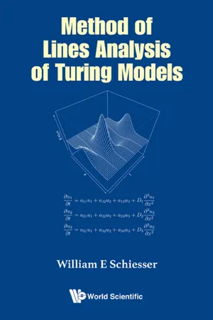
Method Of Lines Analysis Of Turing Models

William E Schiesser

• Publisher: WSPC
• Year: 2017
• ISBN:
  9789813226715
• Topic: Mathematik
• Subtopic: Angewandte Mathematik

-->

This book is directed toward the numerical integration (solution) of a system of partial differential equations (PDEs) that describes a combination of chemical reaction and diffusion, that is, reaction-diffusion PDEs. The particular form of the PDEs corresponds to a system discussed by Alan Turing and is therefore termed a Turing model.

Specifically, Turing considered how a reaction-diffusion system can be formulated that does not have the usual smoothing properties of a diffusion (dispersion) system, and can, in fact, develop a spatial variation that might be interpreted as a form of morphogenesis, so he termed the chemicals as morphogens.

Turing alluded to the important impact computers would have in the study of a morphogenic PDE system, but at the time (1952), computers were still not readily available. Therefore, his paper is based on analytical methods. Although computers have since been applied to Turing models, computer-based analysis is still not facilitated by a discussion of numerical algorithms and a readily available system of computer routines.

The intent of this book is to provide a basic discussion of numerical methods and associated computer routines for reaction-diffusion systems of varying form. The presentation has a minimum of formal mathematics. Rather, the presentation is in terms of detailed examples, presented at an introductory level. This format should assist readers who are interested in developing computer-based analysis for reaction-diffusion PDE systems without having to first study numerical methods and computer programming (coding).

The numerical examples are discussed in terms of: (1) numerical integration of the PDEs to demonstrate the spatiotemporal features of the solutions and (2) a numerical eigenvalue analysis that corroborates the observed temporal variation of the solutions. The resulting temporal variation of the 2D and 3D plots demonstrates how the solutions evolve dynamically, including oscillatory long-term behavior.

In all of the examples, routines in R are presented and discussed in detail. The routines are available through a download link so that the reader can execute the PDE models to reproduce the reported solutions, then experiment with the models, including extensions and application to alternative models.

--> Contents:

• One Dimensional PDEs Introduction
• Eigenvalue Analysis
• Nonlinear Models
• Alternate Coordinate Systems
• Two Dimensional PDEs

-->
--> Readership: Biologists, medical researchers and clinicians, biophysicists, biochemists, biomathematicians, anthropologists, engineers (biomedical, electrical, chemical). -->
Turing Morphogenesis Equations;Partial Differential Equations;Method of Lines0

Chapter 1

One Dimensional PDEs Introduction

Reaction-diffusion (RD) equations are an important class of partial differential equations (PDEs) with broad application in physics, chemistry, biology. Because of this general applicability, they have received extensive discussion.

Various forms of RD PDEs are introduced in this chapter. Numerical methods and associated computer analysis of specific PDE systems are then considered in this and subsequent chapters. The discussion is limited to 2 × 2 (two equations in two unknowns) and 3 × 3 PDE systems, but extensions to larger PDE systems is straightforward.

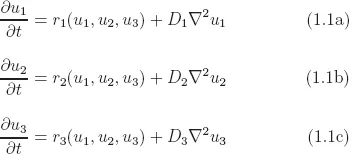
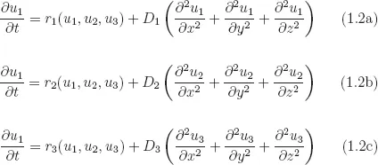
(1.1) Various Coordinate Systems

The following 3 × 3 RD system in coordinate-free form is the starting point for the subsequent discussion of PDEs in specific coordinate systems.

where

u1, u2, u3	dependent variables (concentrations)
t	initial value independent variable, typically time
	Laplacian operator
•	vector product
∇	gradient of a scalar
∇•	divergence of a vector
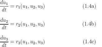
r1, r2, r3	volumetric rates of reaction of u1, u2, u3, respectively

Eqs. (1.1) indicate that the coupling between the equations is through the reaction terms r₁, r₂, r₃. Note that the diffusion terms are linear¹.

Eqs. (1.1) are derived from mass balances ([1], Sec. A1.4). Eqs. (1.1) in Cartesian coordinates x, y, z are

Eqs. (1.2) are parabolic PDEs with reaction (first order in t and second order in x, y, z), This contrasts with hyperbolic PDEs (first order in x and t).

In the subsequent analysis, the 1D special case of eqs. (1.2) is considered (the derivatives in y, z are dropped)². This 1D system is then the basis for the RD PDEs considered by Turing [2].

(1.2) No Reaction Model

For r₁(u₁, u₂, u₃) = r₂(u₁, u₂, u₃) = r₃(u₁, u₂, u₃) = 0, eqs. (1.1) reduce to

i = 1, 2, 3, Eqs. (1.3) are a 3 × 3 system of uncoupled PDEs. In fact, each PDE is just the diffusion equation, also termed Fick’s second law. This special case is used subsequently to test some of the numerical methods and coding.

(1.3) No Diffusion Model

For D₁ = D₂ = D₃ = 0, eqs. (1.1) reduce to

Eqs. (1.4) are a system of ordinary differential equations (ODEs) with no spatial effects, termed a discrete or compartment model. There can be interconnected compartments, each perfectly mixed so that there ...

Table of contents

• Cover
• Halftitle
• Title
• Copyright
• Contents
• Preface
• Chapter 1. One Dimensional PDEs Introduction
• Chapter 2. Eigenvalue Analysis
• Chapter 3. Nonlinear Models
• Chapter 4. Alternate Coordinate Systems
• Chapter 5. Two Dimensional PDEs
• Appendix A1: Spatial Approximations with Finite Differences
• Appendix A2: Spatial Approximations with Splines
• Index