Beams and Accelerators with MATLAB

With Companion Media Pack

Dan Green

• Publisher: WSPC
• Year: 2018
• ISBN:
  9789813237483
• Topic: Sciences physiques
• Subtopic: Physique nucléaire

-->

This book explores a first introduction to particle beams and accelerators. The text uses the suite of tools made available in the MATLAB package. Since many colleges have a site wide license, these tools are often freely available to students. A brief introduction to those tools is made initially. Analogues in classical optics are introduced where useful. The text is compact and focuses on graphical data display and dynamical "movies" as an aid to understanding specific systems. Hands on dialogue using command line inputs, "apps", and "live" tools are stressed. The extensive algebraic steps are subsumed into the associated scripts, where the symbolic math utilities spare the reader from the math manipulations. Both beams and periodic structures are covered. Dispersion, insertions, acceleration and light sources are discussed.

--> Contents:

• Introduction to MATLAB
• Classical Optics
• Uniform Electric and Magnetic Fields
• Dipole
• Quadrupole
• Quadrupole Doublet, Triplet
• Beams
• FODO
• Periodic Structures
• Dispersion
• Insertions
• Low Beta
• Magnet Imperfections and Beam Interactions
• Acceleration
• Medical Applications and Light Sources
• Summary
• Appendices:
  • Inputs for "Plot"
  • Live and App Designer Scripts
  • Initial MATLAB Scripts
  • Useful Trig Identities
  • Collider Accelerator Parameters
  • Radiation Length of the Elements

-->
--> Readership: Graduate students and researchers in high energy physics and accelerator physics. -->
Accelerators;Particle Beams;Optics;Periodic Structures;MATLAB00

Chapter 1

Classical Optics

…the Whiteness of the Sun’s Light is compounded all the Colours where with the several sorts of Rays whereof that Light consists…

— Isaac Newton

Most physicists have more experience with classical optics than with beam optics. For that reason it is useful to recall some facts and definitions from the former.

In classical optics the deviations from the axial line of a series of lens elements can be described by transverse position x and slope m. All transverse excursions are axially symmetric in classical optics, so that simple two-dimensional systems are possible. A matrix can be written that describes the action of some element of the optical system. A ray with an initial position and slope can be traced through the system by making successive matrix multiplications. The matrices for a free space (“drift”) just represent a straight line given the absence of forces and a thin lens, concave or convex (focusing or defocusing), are

In the approximation of a thin lens, the position is not altered but the slope is increased or decreased by an amount x_o/f where f is the focal length. A distance f after the thin lens all incident parallel rays come to a point at x = 0. This is called parallel-to-point focusing. Reversing the process is called point-to-parallel focusing.

The Liouville theorem says that the volume of phase space, x*x′, where the slope m is hereafter replaced by dx/ds = x′ and s is the total path length of the central ray of the system, approximately distance z along the optic axis, is conserved in optical systems consisting of lenses and drift spaces. This requires that the matrix determinant be 1. The area in (x, x′) space is constant, although it may change shape in passing through the optical system.

In point-to-point focusing, the M(1,2) element of the system must vanish. The M(1,1) element is the system magnification in this case. An example is the eye, with small magnification. In the case of parallel to point, M(1,1) = 0. An example is the telescope. For point to parallel, M(2,2) = 0. A familiar example is the flashlight. In classical optics the parallel-to-parallel condition requires M(2,1) = 0 with magnification given by M(2,2). An example is the Galilean refracting telescope. These matrix element conditions follow from the fact that the initial point has x ∼ 0 while an initially parallel beam has x′ ∼ 0. These focal conditions will be seen again when particle beam optics is explored.

This treatment is very simplified. In classical optics there are aberrations due either to the basic lens shape or to variations in the shape because of a manufacturing error. Dispersion is also a common phenomenon, resulting from variation of the focal length with the wavelength of the incident light since the index of refraction depends on wavelength. In beam physics, by analogy, the effects of the electric and magnetic fields depend on the energy of the beam particle itself, which introduces dispersion in the orbits of “off-momentum” particles.

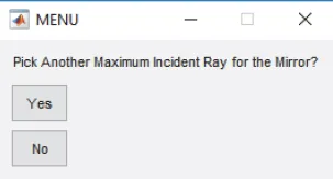
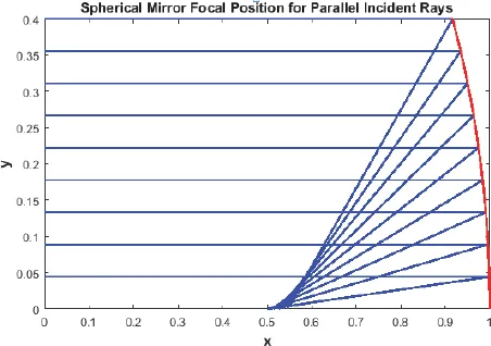
The variations in focal length are illustrated in the script “Spherical_Mirror”. Incident parallel rays are traced through a spherical mirror and the “focal” point is displayed. For a thin lens it is seen that the focus is almost at a point, along the mirror axis at a distance half the radius from the mirror, but for thicker lenses the focal point is smeared out. The “menu” given to the user appears in Figure 1.1. By choosing the largest incident axial ray the user can explore when the spherical aberrations become large. The ray trace for a choice of 0.4 R appears in Figure 1.2. The focal point at x of 1/2 is already becoming smeared.

Figure 1.1:Menu for the script “Spherical_Mirror”.

Figure 1.2:Ray trace for a spherical mirror illustrating the aberration inherent in a spherical mirror. The focal point smearing becomes worse for larger y value incident rays.

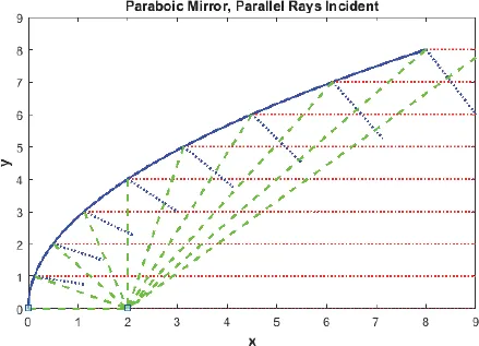
A spherical mirror is easy to grind but has this inherent problem. Astronomical mirrors with a diameter of about 10 m are now operational and larger ones are planned. They are often parabolic in shape, because such a mirror, more difficult to manufacture, has no aberrations for incident parallel rays. There are still focal changes for off-axis rays, called “coma”, but in astronomical applications the incoming starlight is quite nearly axial.

Figure 1.3:Ray trace for a parabolic mirror. The incident rays are red dotted lines, the normals to the parabola are blue dotted lines, and the reflected rays are green dashed lines. The focus is at x = 2.

During the rest of the text, analogies with both classical optics and mechanics, especially simple harmonic motion, will become evident.

Chapter 2

Uniform Electric and Magnetic Fields

An external electric field, meeting it and passing through it, affects the negative as much as the positive quanta of the atom, and pushes the former to one side, and the latter in the other direction.

— Johannes Stark

The topics that will be explored are the motion of charged particles in electric and magnetic fields. These fields are the primary tools that are available to control beams of charged particles. They might make only a single pass through a system, defined to be a beam, or make many passes in stable orbits, as they do in accelerators.

The relativistic equation of motion is the Lorentz force equation, which states that the time rate change of momentum, p, is the force created by the electric (E), and magnetic (B), fields. The charge is expressed in units of the discrete electronic charge e, so that q is an integer. Vectors are indicated by the arrows over the symbols in question.

The magnitude of the velocity is βc, the momentum p, the mass m, and the energy ε. They are connected, using

, by the relationships

The formulae for these quantities will often be used treating c as being equal to 1, as in Eq. (2.2). This may seem disconcerting, but it is standard practice and energy units can be recovered using pc, ε, and mc² with v = βc. For example, ε = γm has the units restored by changing m to mc².

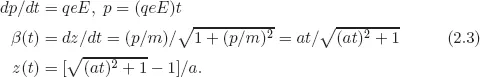
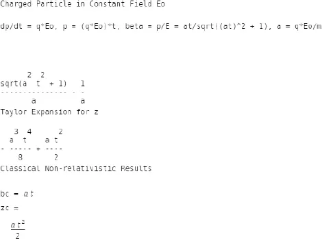
The equation for a uniform electric field — think of motion inside a large capacitor, oriented along the z axis — is solved symbolically in MATLAB in the live script “Uniform_E_Motion”. The script uses the utility “int” to integrate the equation of motion and find z and “taylor” to expand the result in order to find the classical expressions. The utility “eval” is employed to make the numerical plots using the symbolic solutions. The solution for the velocity and position as a function of time is shown in Figure 2.1 and quoted in Eq. (2.3), where a is the classical acceleration qeE/m.

Figure 2.1:Output of the script showing the symbolic solution for z(t) and the Taylor expansion applicable at short times of acceleration.

Since the time derivative of p is constant, p is proportional to t, and β is p/ε, the velocity at long times approaches c while the energy and momentum grow without limit. The classical results are recovered for short times, as is established using the MATLAB utility “taylor” to perform an expansion. The symbolic solution appears in Figure 2.1 and the position as a function of z is displayed graphically in Figure 2.2 for both classical motion and the correct relativistic motion. The script is a “live” one.

The results shown in Figure 2.2 for the velocity and position as a function of time appear dynamically in the script output as “movies”. Each frame is at a fixed time interval...

Table of contents

• Cover Page
• Title
• Copyright
• Preface
• Contents
• Introduction to MATLAB
• Chapter 1. Classical Optics
• Chapter 2. Uniform Electric and Magnetic Fields
• Chapter 3. Dipole
• Chapter 4. Quadrupole
• Chapter 5. Quadrupole Doublet, Triplet
• Chapter 6. Beams
• Chapter 7. FODO
• Chapter 8. Periodic Structures
• Chapter 9. Dispersion
• Chapter 10. Insertions
• Chapter 11. Low Beta
• Chapter 12. Magnet Imperfections and Beam Interactions
• Chapter 13. Acceleration
• Chapter 14. Medical Applications and Light Sources
• Chapter 15. Summary
• Appendix A: Inputs for “Plot”
• Appendix B: Live and App Designer Scripts
• Appendix C: Initial MATLAB Scripts
• Appendix D: Useful Trig Identities
• Appendix E: Collider Accelerator Parameters
• Appendix F: Radiation Length of the Elements
• References
• Index