Phase Transitions for Beginners

Sergei M Stishov

• Publisher: WSPC
• Year: 2018
• ISBN:
  9789813274198
• Topic: Physical Sciences
• Subtopic: Condensed Matter

Written by an experimentalist famous for his discovery of stishovite, with vast experience in phase transition studies, this book is devoted to a description of the continuous and discontinuous phase transitions. It includes chapters outlining the Van der Waals model, hard sphere and soft sphere models of melting, scaling phenomena, renormgroup approach to phase transitions, and experimental examples to illustrate various phase transitions.

Unlike conventional books covering the same topic, this is meant for undergraduate students and experimentalists to understand basic concepts in the physics of phase transitions.

Contents:

• Introduction
• Van Der Waals Model and Critical Phenomena
• Melting
• Step Potential, Quantum Effects, and "Cold" Melting
• The Second Order Phase Transitions and Critical Phenomena
• Bibliography
• Appendices

Readership: For those at the undergraduate to graduate level, to fill conceptual gaps regarding the physics of phase transitions.
Key Features:

• Written by the famous experimentalist who discovered stishovite
• Contains many illustrative experimental examples of various phase transitions
• Includes topics usually not in conventional textbooks and monographs (hard sphere problem, melting, quantum phase transitions, etc.)

Chapter 1

Introduction

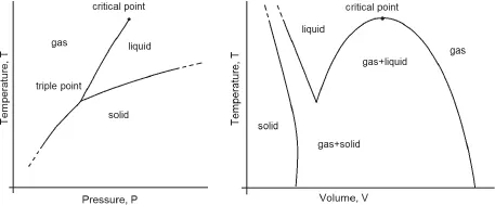
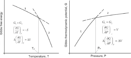
Phase transitions are transitions between different physical states (phases) of the same substance. Common examples of phase transitions are the ice melting and the water boiling, or the transformation of graphite into diamond at high pressures. Figure 1 schematically shows phase diagrams of matter in temperature-pressure (T − P) (a) and temperature-volume (T − V) (b) coordinates.

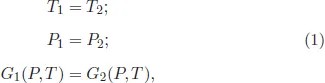
Obviously, these necessarily simplified schemes do not reflect the whole variety of phase diagrams and phase transitions. For example, the melting curve of ice actually has a negative slope (dT/dP < 0), while in Fig. 1 the melting curve is depicted with a positive slope. Moreover, the melting curves can have a maximum, or, due to quantum effects, terminate at absolute zero temperature. The solid-state region (Fig. 1) can include numerous phase transitions associated with changes in their crystalline and electronic structure. Finally, in the case of special forms of interparticle interaction, the critical liquid-vapor point may not appear on the phase diagram of matter. In the above examples, phase transitions are accompanied by abrupt changes in the specific volume and entropy. Such transitions are called phase transitions of the first order, which usually occur at changing an aggregate state of matter and a radical transformation of the crystalline structure of solids. A first-order phase transition is determined by the relations:

Figure 1: Typical form of phase diagram of one-component systems.

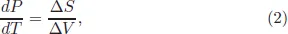
where T, P, G are the temperature, pressure, and the Gibbs thermodynamic potential, respectively. From (1) it is not difficult to derive the Clausius–Clapeyron equation, which defines the slope of the phase equilibrium curves:

where ΔS and ΔV are the volume and entropy changes at the phase transition. Figure 2 illustrates the behavior of the Gibbs thermodynamic potential at a phase transition. As can be seen, the temperature and pressure of the phase transition are determined by the intersection of the potential branches characterizing the coexisting phases of matter. The discontinuities of entropy and volume follow from the crossing of the branches of the thermodynamic potential. Let us pay attention to the fundamental existence of metastable states of matter corresponding to potential regions, which are denoted by the dashed lines.

Figure 2: Behavior of the Gibbs thermodynamic potential at a first-order phase transition.

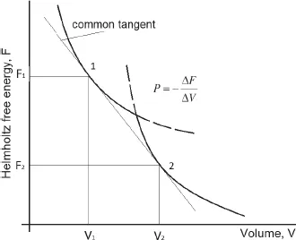
Figure 3: Behavior of the Helmholtz free energy at a first-order phase transition.

In a number of cases it is convenient to consider a phase transition using the Helmholtz free energy as a function of volume. Then, as follows from Fig. 3, the parameters of the first-order phase transition are determined by the common tangent to the branches of the free energy, and not by their intersection, as is the case for the thermodynamic potential. We recall that the general tangent condition means the equality of pressures during the phase transition.

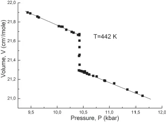
Figure 4: Volume change at the melting-crystallization of sodium, measured by means of a piston piezometer (T = 442.5 K) [1].

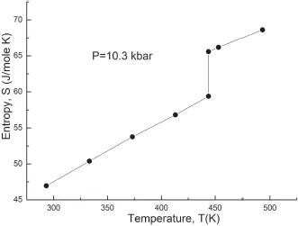
Figure 5: Entropy change at melting of sodium (10.3 kbar). The behavior of entropy is calculated on the basis of P-V-T data [2]. The entropy change is determined using Eq. (2).

The above-mentioned properties of the first-order phase transitions can be illustrated well in Figs. 4 and 5, which characterize the behavior of volume and entropy at melting of sodium, obtained many years ago in the author’s laboratory.

Along with the first-order phase transitions, there is also an extensive group of phase transitions of second order or continuous phase transitions, characterized by a continuous change in the specific volume and entropy, but often accompanied by the peculiarities of heat capacity, coefficient of thermal expansion, compressibility, etc. The second-order phase transitions include transitions associated with an emergence of magnetism, superconductivity, superfluidity, orientational order, etc.

This classification, proposed in due time by P. Ehrenfest, operates with the orders of the derivatives of thermodynamic potential that experience discontinuities at the phase transition. Eliminating the uncertainty in Eq. (2) for ΔS = 0 and ΔV = 0 by the L’Hˆopital’s rule, Ehrenfest proposed equations relating the slope of the phase transition curve to discontinuities in the heat capacity, compressibility, and thermal expansion coefficient [5].

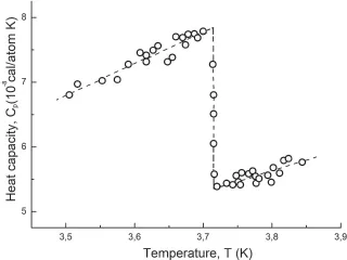
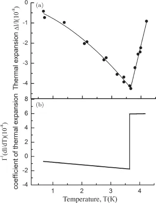
Subsequently, it was found that, for the most part, in the phase transitions of second order, the divergence of the corresponding quantities is observed as a result of fluctuation effects. Nevertheless, Ehrenfest’s classification and its equations not only retain their significance as a way of systematizing phase transitions, but can also be used in analyzing phase transitions with weakly developed fluctuations, such as superconducting phase transitions, occurred in the conventional superconductors. The results of measurements of the heat capacity and thermal expansion of white tin, demonstrating completely “Ehrenfest” behavior, are displayed in Figs. 6 and 7.

It should also be pointed out that there exists in some sense an intermediate group of phase transitions — the so-called first-order phase transitions close to the second-order ones. In this case, the phase transition initially occurs according to the scenario of the continuous transitions, but somewhere, not reaching the virtual point of the second-order phase transition, ends abruptly as a first-order transition. The phase transitions in ferroelectrics BaTiO₃ and KH₂PO₄ (KDP) can serve as examples. It should also be noted that in two-dimensional and quasi-two-dimensional systems, Kosterlitz–Thouless transitions can be observed that are not accompanied by distinct features of thermodynamic quantities. Consequently, they are dropping out of the Ehrenfest’s classification.

Figure 6: Heat capacity of tin in the region of superconducting phase transition [3].

Figure 7: Linear thermal expansion of a single crystal of tin in the region of the superconducting phase transition [4].

Chapter 2

Van der Waals model and critical phenomena

2.1.Van der Waals equation

The year of 1869 should be considered as a starting point in the development of scientific ideas about phase transitions, when Thomas Andrews unveiled his studies of critical phenomena in CO₂. Four years later, van der Waals created his famous molecular theory of critical phenomena, which has not lost its significance up to the present time. In view of the particular importance of this theory, its main points are outlined.

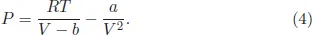
The standard van der Waals equation has the form:

It is convenient to rewrite (3) as:

The original idea of van der Waals was to represent the interparticle interaction in the form of an infinite repulsion at some finite distance and a very long-range attract...

Table of contents

• Cover
• Halftitle
• Title
• Copyright
• Contents
• Foreword
• 1. Introduction
• 2. Van der Waals model and critical phenomena
• 3. Melting
• 4. Step potential, quantum effects and “cold” melting
• 5. The second order phase transitions and critical phenomena
• Bibliography
• Appendix