Fractalize That!

A Visual Essay on Statistical Geometry

John Shier

• Publisher: WSPC
• Year: 2018
• ISBN:
  9789813275188
• Topic: Mathematics
• Subtopic: Geometry
• Index: Mathematics

Fractalize That! A Visual Essay on Statistical Geometry brings a new class of geometric fractals to a wider audience of mathematicians and scientists. It describes a recently discovered random fractal space-filling algorithm. Connections with tessellations and known fractals such as Sierpinski are developed. And, the mathematical development is illustrated by a large number of colorful images that will charm the readers.

The algorithm claims to be universal in scope, in that it can fill any spatial region with smaller and smaller fill regions of any shape. The filling is complete in the limit of an infinite number of fill regions. This book presents a descriptive development of the subject using the traditional shapes of geometry such as discs, squares, and triangles. It contains a detailed mathematical treatment of all that is currently known about the algorithm, as well as a chapter on software implementation of the algorithm.

The mathematician will find a wealth of interesting conjectures supported by numerical computation. Physicists are offered a model looking for an application. The patterns generated are often quite interesting as abstract art. Readers can also create these computer-generated art with the advice and examples provided.

Contents:

• Introduction: Space-Filling Patterns
• Squares and Rectangles
• Triangles and Diamonds
• Discs and Circular Arcs
• Mixed and Irregular Shapes
• Examples
• The Statistical Geometry Algorithm
• The Area–Perimeter Algorithm
• Statistical Geometry in One Dimension
• Do It Yourself

Readership: Students, mathematicians, physicists, professionals, and the general public who are interested in the fractal art of statistical geometry.
Key Features:

• The book brings together information from the few published papers and unpublished material reported here for the first time
• This is the first book-length description of the subject
• Examples of the use of the algorithm for decorative art
• A visual feast

Chapter 1

Introduction: Space-Filling Patterns

Ways of filling space with tiles have been known since ancient times. If we have square or rectangular tiles it is easy to fill any spatial area by simply placing more and more of them side-by-side. Millions of bathrooms and shower stalls have tiled walls of this kind. With a particular area to be filled and a particular tile size, only a finite number of tiles are needed to cover the area. There are many other ways to cover an area with tiles having the shapes of triangles, hexagons, etc. The formal word for a tile pattern is tessellation.

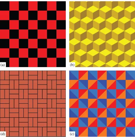
Figure 1.1 shows several simple tessellations. If all of the tiles have the same color, we lose all sense of separate pieces, so it is traditional to use different colors in a regular sequence. The checkerboard of Fig. 1.1(a) is one of the most common examples; it uses two colors. Another common example is shown in Fig. 1.1(b). It uses a diamond having 60° and 120° corner angles and requires three colors. The diamonds have three orientations which are rotated 120° from each other. One must color the three orientations differently in order to see the pattern, and with a suitable choice of shading the image has a strong three-dimensional illusion — the eye perceives polyhedral bumps sticking out of the plane.

Fig. 1.1. Tessellations. (a) A checkerboard formed from squares. (b) “Tumbling blocks” made by tiling 60°–120° diamonds. (c) A tiling using 45° triangles; an example of a Truchet tiling. (d) A pattern sometimes seen in brick sidewalks.

Figure 1.1(c) shows a tessellation made with symmetric triangles having two 45° corners. Two such triangles joined in a square is called a “Truchet tile”. There are four possible orientations for the triangles, shown by the four colors used. A huge number of repeating patterns can be made with these tiles, and mathematical studies of the possible arrangements have been done. The paired rectangles pattern shown in Fig. 1.1(d) is often seen in brick sidewalks, and only works if the bricks have a width half their length.

It can be shown mathematically that there are 17 possible symmetries [1] for planar tessellations where every piece repeats periodically as we move left–right and up–down as in Fig. 1.1. In the 1970s, the mathematical physicist Roger Penrose showed that it is also possible to take two simple polygonal shapes and fit them together to fill all space in a manner which does not repeat: a non-periodic tessellation.

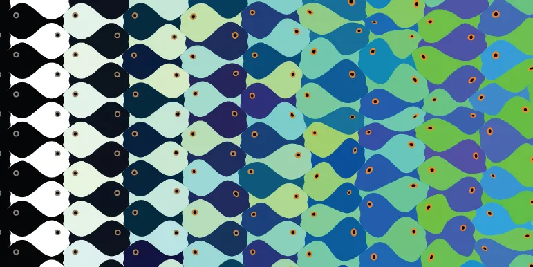
Quite interesting uses for tessellations were invented by the Dutch artist Maurits Escher in the late 20th century [2]. Escher’s idea was to distort the sides of the tiles in such a way that we retain the basic space-filling property, while teasing the shape into that of a familiar object such as a fish or bird. Figure 1.2 shows an example of a fish tessellation with a twist. At the left, the fishes are simple black and white repeating shapes. As we move to the right, the fishes gradually acquire unique colors and become distorted into shapes which are no longer the same, while they remain space-filling. The fishes at the right seem to be trying to swim out of the picture.

Tessellations fill a finite region of the plane with a finite number of shapes. In the early 20th century, geometric constructions were invented which fill a finite region with an infinite number of regular shapes. One of the best known of these is the Sierpinski [3] triangles.

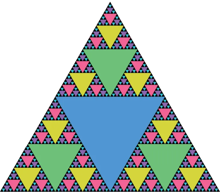
The construction of Fig. 1.3 begins with an empty black triangle. An oppositely-pointing blue triangle is placed in the middle of it, creating three new smaller empty triangles in the corners. We then proceed to place new, smaller green triangles in these empty spaces, which create yet more empty triangles, which in turn get yet smaller light green triangles placed, etc. The procedure follows a regular pattern of “generations” or “recursions”, with each new generation having three times more triangles than the previous one, each with a side length half that of the previous generation. Figure 1.3 shows six generations, each with a different color, and it can be seen that the remaining unfilled black area is already quite small.

Fig. 1.2. A tessellation constructed with a fish shape. The regularly repeating symmetric black–white shapes at the left progressively shift to distorted and colored shapes at the right.

Fig. 1.3. The 6th generation of a Sierpinski fractal construction which fills a black triangle with an infinite number of smaller triangles.

Those familiar with Sierpinski’s work will see that I have reversed the usual procedure in which a filled triangle is successively emptied by cutting out smaller triangles. The “cutting out” method is used in mathematics, while the “adding” method described here has been adopted by physicists in studies of how material particles pack together [4–6]. The additive approach is much more attractive for visual art. Where usage differs we will follow the physics conventions.

The Sierpinski triangles never quite fill the whole region; there is always some area left over even after a huge number of generations. We call the left-over region the gasket. It is easy to see that even after a large number of generations, the total area of all the inserted triangles remains finite, with a limiting value equal to the area of the initial triangle. If, however, we consider the total perimeter of the triangles, it grows without limit. This paradoxical behavior is characteristic of fractals [3]. The construction of a fractal involves ever-finer fracturing or fragmentation of the region which is to be filled. This fragmentation property of a fractal can be described mathematically in terms of a fractal dimension D which is not an integer [3].

Mathematicians make a distinction between a disc and a circle. A disc contains all of the points within a circular boundary. A circle contains only the points on the curved line. We follow this convention in the book.

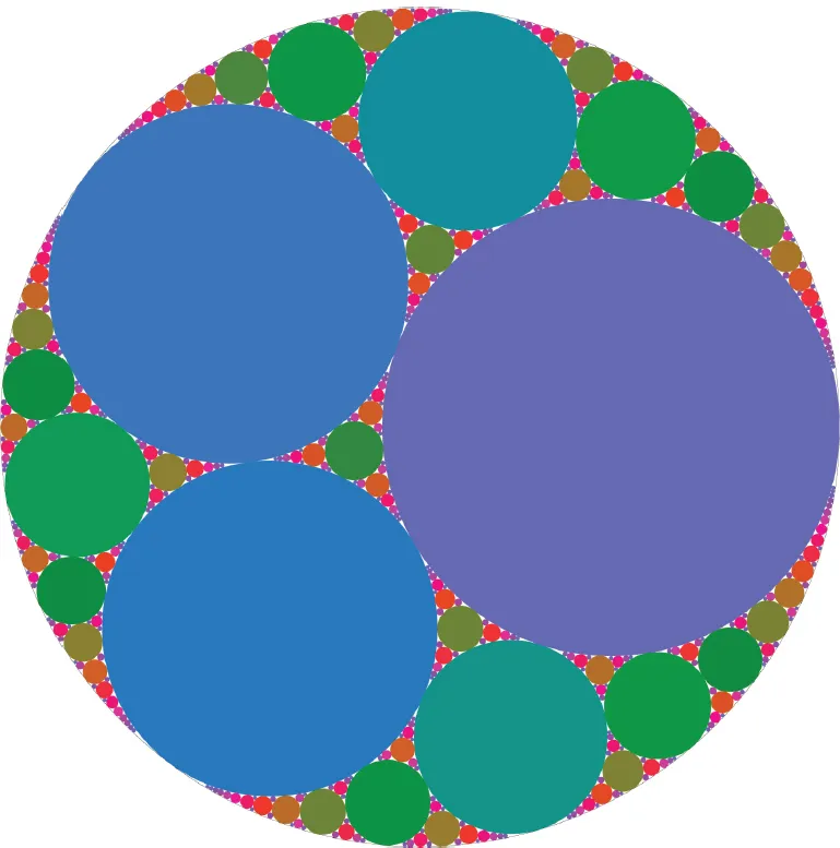
Most people will look at a circle and say “There is no way to completely fill a planar region with discs. They don’t fit together smoothly.” But if we are willing to consider the use of an infinite number of discs, it is possible to make constructions which are space-filling “in the limit” where we allow an infinite number of ever-smaller discs. These patterns have received the name “Apollonian circles” and are of several kinds depending on what bounding region we set out to fill. Figure 1.4 shows an example.

Fig. 1.4. A touching-discs construction which fills a bounding circle “in the limit” with an infinite number of small discs. It has been given the name “Apollonian circles” after the ancient Greek mathematician Apollonius who showed that given any three circles, it is possible to find a fourth circle which is tangent to all of them. It makes an interesting comparison with Fig. 1.6 and Fig. 4.1 in Chapter 4. Log-periodic color. Data courtesy of Steve Butler.

The circles are placed by taking existing circles three at a time and constructing smaller circles which are tangent to all three. Like the Sierpinski triangles, the Apollonian circles have a fractal dimension D which is not an integer [3].

In the fractal space-filling patterns described so far, every fill region has an exact size and position. The fill region shapes are the simple shapes of elementary geometry. In what follows, we will see that if we are prepared to abandon this regularity, it is possible to create space-filling random fractals [7, 8] where the sizes of the fill regions follow a regular rule but their positions do not. The surprise is that it is apparently possible to do this for any fill region shape, including quite odd “blobby” ones unknown to any geometric text.

Before taking up the images generated by this new technique, it is desirable that the reader understand something about how they are created. Without some insight into the process, it is difficult to grasp what is going on. The first step is to assume a spatial region to be filled, which has an area A. It is usually a square or rectangle in the examples here, but in principle it can be any shape. It is to be filled with ever-smaller fill regions, and the next step is to generate the sequence of areas for these regions according to a mathematical rule called a power law. In a particular example, the sequence might run 1.6870, 1.1277, 0.8851, … and keep on getting smaller. These numbers can be thought of as areas in square inches or other convenient units. We omit details, but the sum of these areas (to infinity) is just the total area A which is to be filled. Many such area sequences are possible, with the details depending upon the choice of two numbers used in generating them — the power-law exponent c and the starting point N. A mathematical account of the algorithm can be found in Chapter 7.

After finding the area sequence, we choose a particular fill region shape (such as a circle, square, or crescent). We proceed with the areas in order of size, beginning with the largest. For the largest area we find the fill region’s linear size. If the fill region is a disc, the linear dimension of interest will be the i-th radius, which we can find from the formula

from elementary mathematics. Other fill region shapes have more complicated formulas. The first shape is placed at random within the region to be filled, such that it does not touch or overlap any of its boundaries. This step is called the initial placement.

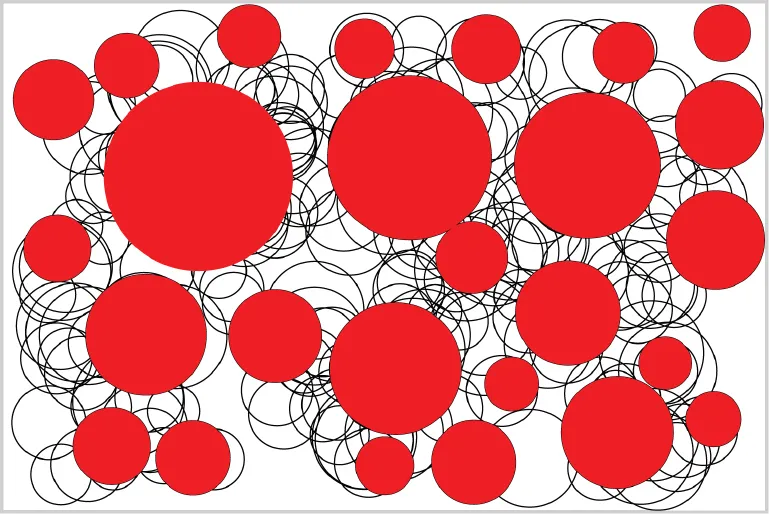
Fig. 1.5. An illustration of the process for discs in a rectangle. Each black-line circle shows a random trial. After 25 discs were placed, a red disc was drawn at the location of each successful trial (placement). It is evident that there were many unsuccessful overlapping trials.

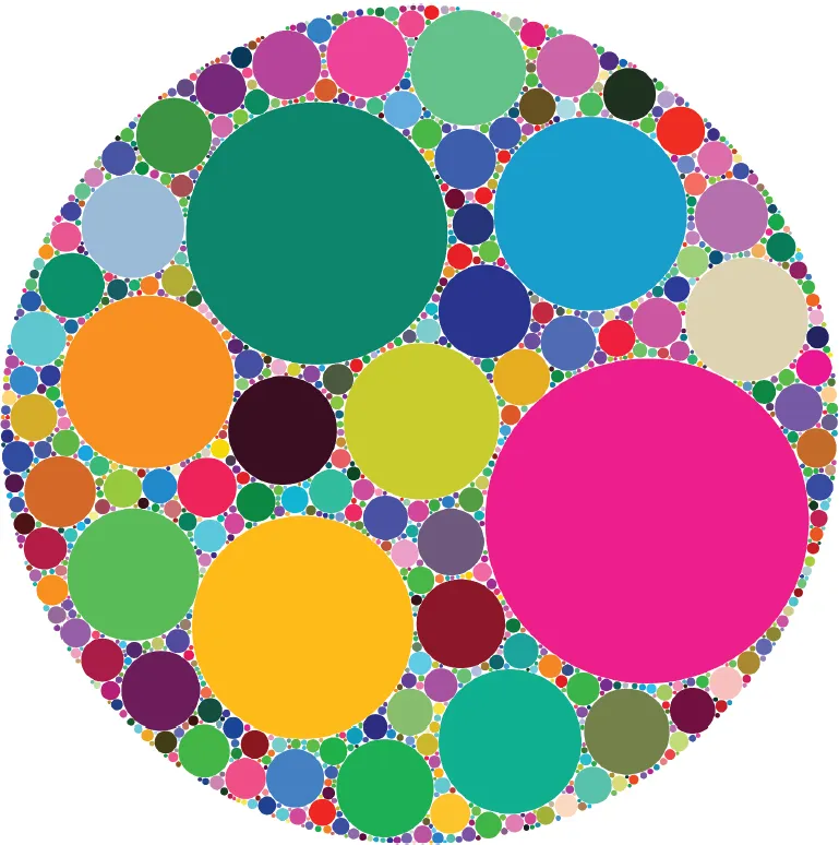
Fig. 1.6. A random disc fractal with a circular boundary. The colors are random, but done in a way that excludes very dark and light colors. c = 1.49, N = 3, 1200 discs, 95% fill, and white gasket. Note the similarity to Fig. 1.4.

We then proceed with the following fill regions (shapes) in order of decreasing size. For each fill region, we find its linear dimension(s) and then try it at a random place within the region to be filled. This random step is called a trial, and at this random location the shape may overlap with some previously placed fill region or with a boundary, in which case the trial fails and we do another trial with the same fill region at a diff...

Table of contents

• Cover
• Halftitle
• Title
• Copyright
• Preface
• About the Author
• Acknowledgments
• Contents
• Chapter 1 Introduction: Space-Filling Patterns
• Chapter 2 Squares and Rectangles
• Chapter 3 Triangles and Diamonds
• Chapter 4 Discs and Circular Arcs
• Chapter 5 Mixed and Irregular Shapes
• Chapter 6 Examples
• Chapter 7 The Statistical Geometry Algorithm
• Chapter 8 The Area–Perimeter Algorithm
• Chapter 9 Statistical Geometry in One Dimension
• Chapter 10 Do It Yourself
• References
• Index