Survey Research

Roger Sapsford

• Publisher: SAGE Publications Ltd
• Year: 2006
• ISBN:
  9781446237335
• Edition: 2
• Topic: Social Sciences
• Subtopic: Social Science Research & Methodology
• Index: Social Sciences

This much-anticipated Second Edition presents an informative and accessible account of survey research. It guides the reader through the main theoretical and practical aspects of the subject and illustrates the application of survey methods through examples. Thoroughly revised and updated, it presents:

• Concise and analytic coverage of multivariate analysis techniques
• A new chapter giving theoretical and practical advice on the stages involved in constructing scales to measure attitude or personality
• An account of using materials on the internet
• Concise introductions and summaries to all chapters

This book will prove to be equally useful for students conducting small research projects in the social sciences or related professional/applied areas, researchers planning systematic data collection for applied purposes and policy makers who want to understand and analyse the research with whose conclusions they are presented.

Part D

EXPLORING DATA

9

KEEPING IT SIMPLE: TABULAR ANALYSIS

---

In the first of three chapters on the analysis of survey data we shall look at the simplest form of complex analysis, using tables to explore relationships.

---

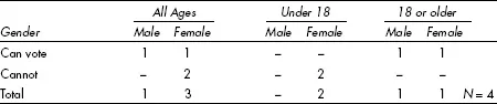
No paradox is intended here in the juxtaposition of ‘simple’ and ‘complex’. Tables are just about the simplest way of describing a sample: they just present the counts. In a given family, suppose that three-quarters of the members are female, and half – all female – cannot vote. There is a clear association at the level of the sample, therefore, between gender and being able to vote. In reality, however, gender is not the important factor here; half the family are under the age of 18 – both females, as it happens – and there is a perfect association between age and having the franchise (Table 9.1). This is what I mean by complex analysis – being able to reason from apparent associations in samples to actual associations in the population, taking account of more than two variables and allowing for sampling error – and all this can be done using tables.

Table 9.1 Gender, voting and age in one family

Significant association in tables

---

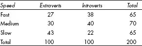
There is little that can be concluded from Table 9.1; it does not contain enough cases to allow much in the way of analysis. Consider Table 9.2, however, which looks at measurements taken from a mythical random sample of 200 students in a particular university. The sample has been divided at the mid-point into the 100 more extravert students and the 100 more introverted – on the basis of questionnaire scores, let us say – and their performance on a simple reaction-time task has been used to split them into three roughly equal groups – the slowest 65, the fastest 65 and the 70 people in the middle. There are enough cases here for conclusions to be drawn, so what do we want to say about the table?

Table 9.2 Extraversion and speed of reaction in a mythical sample

There is an obvious relationship, in this sample, between extraversion/introversion and speed of reaction time. There are about twice as many extraverts as introverts in the ‘slow’ third, and substantially more introverts in the other two rows. (The two columns have the same total, so we can validly compare them.) This is factual information and needs no testing; it is the case that the extraverts are on average slower than the introverts in this sample. What can we say about the population from which the sample is drawn, however?

Well, first we have to acknowledge that the sample is not likely to be representative of the general population, because it consists entirely of students, who tend to come from a very restricted age range and are likely to differ from the rest of the population in terms of background, education and motivation. We cannot even treat the sample as representative of students as a whole, because it comes from a single university and is therefore covertly selective. The best we would say is that the results may be suggestive but would need checking on different samples.

As a sample of the cohort of students in this one university this group might be reasonably representative, as it was randomly chosen. Even a random sample might not be representative, however; unrepresentative samples can be drawn by random means (see Chapter 3). Given the relationship between extraversion/introversion and reaction times in this sample, how likely is it that there is a similarly strong relationship in the parent population? How likely is this to be an untypical sample drawn by chance from a population in which the relationship does not hold? This is the question of statistical significance, discussed in earlier chapters, and it can be decided by statistical means. The statistic we shall be using mostly in this chapter is chi-squared (written c², where c is the Greek letter ‘chi’, pronounced ‘kye’). It involves model-fitting: working out what the table would look like if there were no association between the variables, and then assessing how different the observed figures are from these ‘expected’ ones. If the difference is sufficiently large the null hypothesis of ‘no difference’ will be rejected and we shall assert that the sample difference probably reflects a real difference in the population – with a designated probability of being in error.

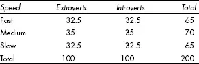
If there is no association between the two variables – if your score or position on one does not predict where you will score on the other – then the numbers in each row, or each column, will be distributed in the same proportions as the table’s marginal totals. In Table 9.2 we have equal numbers of extraverts and introverts, so if there is no association – if extraversion is not predictive of reaction time – then we should have equal numbers in each row as well. These are the expected values, on the basis of the null hypothesis – the model of ‘no association’. The expected vales associated with Table 9.2 are shown in Table 9.3.

You might like to work them out for yourself before looking at Table 9.3. (Hint: don’t worry if some of the answers are not whole numbers.)

Table 9.3 Expected values for Table 9.2

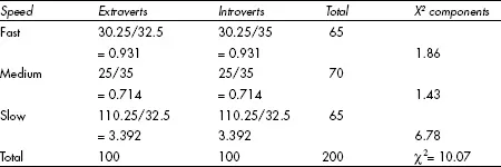
Now, our measure of difference between the ‘null hypothesis’ model and the observed (actual) figures starts with subtracting the expected value from the observed one. So, in the first cell we have an observed value of 27, an expected value of 32.5 (half of 65) and so a difference of -5.5. Next we square this figure, so that larger differences have proportionately more impact on the result than smaller ones, giving a new figure of 30.25. Finally, it is evident that the importance of a difference depends on how big the numbers were – the difference between 7 and 5 is more important than the difference between 102 and 100 – so we scale the result by dividing by the expected value. This gives us a chi-squared value of 30.25/32.5 = 0.931 (to three decimal places). This is the first component of the statistic. You now do precisely the same for every cell and add up the resulting figures, to obtain the overall value of chi-squared for the table, which is 10.07. The calculations are shown in Table 9.4.

Again, you might like to do the calculation for yourself before looking at Table 9.4.

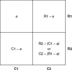
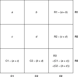
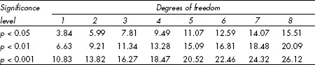
Now we look up the value of chi-squared in a special table of probabilities, to find the significance level of the result. A small version of the table is reproduced as Table 9.5. We need one more concept before we can do this, however – the notion of degrees of freedom. In a table with only four cells – two rows and two columns – we can work out every figure in the table, given the marginal totals and one other number (see Figure 9.1). The table is therefore said to have one degree of freedom. With a three by three table (Figure 9.2) we need four figures, as well as the marginal totals, before we can work out the rest by subtraction, so the table has four degrees of freedom. The general rule is that the number of degrees of freedom is given by (R–1)(C–1), where R is the number of rows and C is the number of columns.

Table 9.4 Calculating chi-squared for Table 9.2

Figure 9.1 One degree of freedom

So how many degrees of freedom does Table 9.2 have?

There are three rows and two columns in Table 9.2, so there are (3–1) (2–1) = 2 degrees of freedom. This is the final piece of information we need to determine the significance of the association between the two variables. We look at Table 9.5, in the column for two degrees of freedom, and we find that we need a chi-squared value of 5.99 or higher for significance at the 0.05 level, and 9.21 or higher for significance at the 0.01 level. Our chi-squared value of 10.07 for Table 9.2 is therefore significant at the 0.01 level, so we can assert that we ought to get a sample with this large an association, from a population where there is no association, less often than one time in a hundred (p < 0.01).

Figure 9.2 Four degrees of freedom

Table 9.5 Critical values for the chi-squared statistic

An important limitation on the use of chi-squared is that it is not valid – it does not necessarily give the right answer – if numbers are too small. A usual rule of thumb is that every expected value must be at least 5, though in large tables a few expected values less than 5 can be tolerated provided they are randomly scattered. (If they form a pattern – run along a row or column – then you probably need to combine categories to increase the expected values.)

There are a number of other tests of the significance of association in tables which are in common use. Two of them are briefly described in Box 9.1, along with a summary of information about chi-squared.

---

Box 9.1 TESTS FOR SIGNIFICANT ASSOCIATION IN TABLES

Chi-squared (χ²):

This is a useful general-purpose test, applicable to any size of table provided that expected values are at least five in each cell (or most of them, on large tables). To calculate: for each cell, compute χ² = (O – E)²/E, where O is the observed value in the cell, and E is the expected value under the null hypothesis of no association, calculated by dividing the row total by the proportion of cases in the column (or the other way about – whichever is most convenient).

When working with 2 × 2 tables (two rows, two columns) the value of chi-squared should be reduced slightly by applying a correction for continuity. The simplest way to calculate the corrected chi-squared is to use an overall formula rather than calculating cell chi-squared. If we label four cells of the table as A to D (A and B in the top row, C and D in the bottom), then the corrected chi-squared is given by

χ² = ((A – D) -1)²/(A + D),

taking the absolute value of (A – D) – that is, ignoring any minus sign.

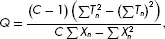
McNema’s Q

This is used where we have dichotomous information (‘yes/no’, ‘pass/fail’) for a number of individuals (N) on a number of measures/questions (C), or for N individuals under C conditions for a single measure, or N sets of C matched individuals on a single item. The formula is

where T_n is the total in the nth column and X_n is the total in the nth row.

Provided N is larger than abo...

Table of contents

• Cover Page
• Title Page
• Copyright Page
• Contents
• Preface
• List of Examples
• List of Boxes
• PART A INTRODUCTION
• PART B THE SIZE OF THE PROBLEM
• PART C OPINIONS AND FACTS
• PART D EXPLORING DATA
• PART E FINISHING UP
• References
• Name index
• Subject index