Geographic Health Data

Fundamental Techniques for Analysis

Francis Boscoe

• Publisher: CAB International
• Year: 2013
• ISBN:
  9781789244045
• Topic: Medicine
• Subtopic: Public Health, Administration & Care

Focussing on proven techniques for most real-world data sets, this book presents an overview of the analysis of health data involving a geographic component, in a way that is accessible to any health scientist or student comfortable with large data sets and basic statistics, but not necessarily with any specialized training in geographic information systems (GIS). Providing clear, straightforward explanations with worldwide examples and solutions, the book describes applications of GIS in disaster response.

1 Points, Lines and Polygons

Francis P. Boscoe*
Department of Epidemiology and Biostatistics, University at Albany, New York, USA

1.1 Introduction

Any natural or human-created feature on or near the earth’s surface can be represented as a zero-, one- or two-dimensional object. In this book we refer to these objects, respectively, as points, lines and polygons; commonly encountered synonyms include nodes, arcs, and areas, respectively. (While it is also possible to represent features as three-dimensional objects, this is rarely called for in public health, and is beyond the scope of this book.) The type of object that is chosen to represent a particular feature depends on the scale of interest. At the scale of a nation, rivers are typically represented as lines and cities as points, but at a fine scale both can be represented as polygons.

The relationships between points, lines and polygons are the domain of a branch of mathematics and computer science known as computational geometry. Scientists working in this sub-field concern themselves with finding efficient algorithms for computing these relationships. These algorithms form the core of geographic information system (GIS) software packages, and are also integral to the rendering of computer graphics in films and video games and navigation problems in robotics.

University courses in GIS tend to gloss over these algorithms. Instead, students are shown the menus or toolbars needed to compute and display the underlying relationships; the inner workings of the software remain a mystery. As discussed in the introduction, this approach has its limitations.

The purpose of this chapter is to provide a glimpse of the inner workings of GIS software by reviewing some of the basic algorithms governing the relationships of points, lines and polygons. These relationships are universal and can be implemented in just about any programming language or statistical software package that one chooses. When I receive GIS-related questions in my capacity as an employee of a state health department, it is often the case that the questioners possess the knowledge and skills needed to answer the question, but have been blinkered by the belief that they lacked some essential piece of specialized software.

While the specialized journals within the sub-field of computational geometry can be densely mathematical, many of the basic concepts require only rudimentary spatial thinking and common sense, and can be communicated with a minimum of mathematical notation. That is the approach I take here. I also focus on more easily explainable solutions, as opposed to optimal solutions, to the extent that they differ. For a more rigorous treatment of the material presented here, I recommend the textbook Computational Geometry: Algorithms and Applications (de Berg et al., 2000).

1.2 Referencing Locations

Before continuing any further, it is first necessary to discuss how locations on the earth’s surface are expressed. This book mainly makes use of latitude and longitude. Latitude describes the distance north or south of the equator, with values ranging from 0 degrees (0°) at the equator to 90° at the poles. By convention, values in the northern hemisphere are positive and those in the southern hemisphere are negative. The distance from the equator to the poles is very close to 10 million m (indeed, the metre was originally defined in the 18th century as one ten-millionth of this distance), so a degree of latitude is about 111 km or 69 miles, about an hour’s drive on an empty highway. This is true at all locations on the earth, as latitude lines are parallel.

Longitude describes the distance east or west of the prime meridian, a line connecting the north and south poles that passes through England, France, Spain and several West African countries. Values range from 0° to 180°, with positive values east of the prime meridian and negative values west of it. As longitude lines are not parallel, the distances between them vary – distances are greatest at the equator and shrink to zero at the poles, where all longitude lines converge. A simple way to find the distance between two longitude lines at a given latitude is to multiply 111 km by the cosine of the latitude. For example, at 45° north or south latitude, a degree of longitude is 111 times the cosine of 45° (0.707), or about 79 km (49 miles). Traditionally, latitude and longitude values were recorded in units of degrees, minutes (′) and seconds (″), with 60 minutes per degree and 60 seconds per minute. More recently, it has become standard practice to use decimal degrees (for example, 60.4167° rather than 60°25′). Clearly, this is more convenient in our decimal-based maths system.

The use of latitude and longitude, or any coordinate reference system, requires some assumptions about the shape of the earth. The earth is very close to a perfect sphere, and calculations and measurements based on this assumption will yield only small errors, which are acceptable for many purposes. However, because some measurements, such as property surveys, demand the greatest possible precision, more exact definitions of the earth’s shape have been widely developed and used over the last two centuries. Historically, these have been country or region specific. More recently, the widespread adoption of the global positioning system (GPS) has encouraged the use of a single definition of the earth’s shape applicable to the entire globe, specifically, the World Geodetic System of 1984 (WGS84). Locations in WGS84 typically differ by tens of metres from the earlier systems. Most commercial GIS software can make the necessary conversions, though as time goes on, data sets using the earlier reference systems are encountered less frequently. In any event, issues of geodetic precision are seldom relevant to public health data sets. This topic is covered in more detail in Chapter 5.

Besides latitude and longitude, the most often seen coordinate system in current use is the Universal Transverse Mercator (UTM). The UTM system divides the inhabited earth into 60 zones of 6° of longitude each. Within each zone, distortion of distance is less than one part per thousand. Locations are given as x-and y-coordinates called eastings and northings, in units of metres. In the northern hemisphere, the northing describes the distance from the equator; in the southern hemisphere, it describes the distance from the South Pole. The easting describes the distance from the central meridian within the UTM zone. To avoid negative numbers, the central meridian is assigned the easting value 500,000. Hence, the location of the Sydney Opera House can be given as 56S/N 6,252,309/E 334,897, where 56 is the zone number, S stands for the southern hemisphere, N and E stand for northing and easting, 6,252,309 is the distance from the South Pole in metres (and thus about 62.5% of the distance from the South Pole to the equator), and 334,897 indicates that the point is about 165 km west of the central meridian of zone 56 (obtained by subtracting 334,897 from 500,000).

The mathematics of converting latitude and longitude to UTM or vice versa are quite involved, but most GIS software has this functionality built in. For those working outside a GIS, there are a number of calculators online, including one I have written for SAS software, which can be accessed by visiting www.sascommunity.org and searching on the term ‘UTM’ (sascommunity.org, 2013).

1.3 Point in Polygon

I begin our brief tour of useful geographic algorithms with the point-in-polygon relationship. Given a set of point locations, it is often helpful to know which polygons, if any, the points are contained within. This is most commonly encountered in the calculation of disease rates for geographic areas. A disease rate is simply the number of disease cases divided by the population. Disease cases are often recorded as point locations, typically at the residence at the time of diagnosis, while populations are expressed as polygons, such as states or districts or census units. The point-inpolygon relationship is illustrated in Fig. 1.1, which shows an irregular 17-sided polygon and three points of interest, X, Y and Z. Obviously, points X and Z are inside the polygon, while Y is not, but how does GIS software know this?

The answer is obtained by extending a ray from the point of origin in any direction, and counting the number of intersections with the polygon concerned. For this reason, this method is known as the ray-tracing method. If the number of intersections is odd, the point is inside the polygon; if the number is even, the point is outside. This property, often simply called the ‘even–odd rule’, is a cornerstone of computer graphics. In Fig. 1.1, the rays have been extended to the left in the 17-sided polygon. From points X and Z there are three intersections, so these points must be inside the polygon. From point Y there are four intersections, so it must be outside.

Computer software keeps track of the number of intersections of the ray by comparing the locations of the nodes forming each of the 17 sides of the example polygon with each of the three points of interest. If a pair of nodes both have a higher x-coordinate than one of the points of interest, then that line segment of the polygon is to the right of the point of interest and so there is no intersection with the ray. For point X, this is true of sides CD, DE, EF, MN and NO. A second test is applied to the y-coordinates to eliminate those segments that are entirely above or below the point of interest. For point X, this is true of sides AB, BC, HI and QA, among others. What remains are the sides that do intersect: FG, GH and JK. One way to summarize this process is through pseudocode, a list of computer-code-like instructions that is not written in any particular computer language, and may even be written in plain English. For example, plain-English pseudocode for the point-in-polygon match could be written as:

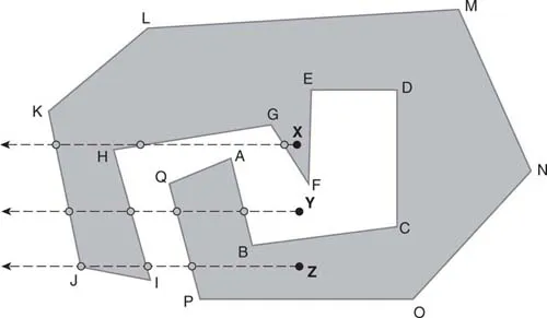
Fig. 1.1. Determining whether a point falls within a polygon.

• For each point of interest, do the following:

• For each line segment within the polygon, do the following:

• Perform x-coordinate test:

• If the x-coordinates of both points comprising the line segment are greater than the x-coordinate of the point of interest, then there is no intersection

• Otherwise, perform y-coordinate test:

• If the y-coordinates of both points comprising the line segment are greater than or equal to, or less than, the y-coordinate of the point of interest, then there is no intersection

• Otherwise, the segments intersect:

• Increase intersection count by 1

• If final intersection count is odd, then the point is in the polygon

• Otherwise, the point is outside the polygon

Note the italicized phrase ‘or equal to’ in the description of the y-coordinate test. This was added to address the situation where a ray intersects a node exactly, as in the case of point J in Fig. 1.1. As the y-coordinates of points Z and J are equal, neither IJ nor JK would count as an intersection using the original logic. Under this revised logic, JK counts as intersecting but IJ does not, thus yielding the correct result. This special situation is known as a degenerate case. For most algorithms, it is useful to first find a general solution and then to modify it to incorporate degenerate cases. Another degenerate case not yet covered by this algorithm describes the situation when a point lies on the exact edge of a polygon. Should such a case be counted as inside, outside or neither? One could argue that this instance could be safely ignored as it is highly unlikely to occur – people are residents of particular countries, provinces and so on, and it is not possible to occupy their exact borders. However, in my experience, if something can occur in a spatial data set, it probably will, and so good programming practice dictates that this instance be accounted for by the algorithm as well. Because I would be suspicious about the accuracy of any such points, I would be inclined to place them into a special category for later manual review and correction.

Geographic coordinates tend to be reported with very high precision, often to at least six decimal places, or 11 cm of latitude. While such precision is rarely scientifically appropriate, it does have the advantage of minimizing degenerate cases; here as long as all points are positioned at least 11 cm from all polygon edges, there will be no problems.

The pseudocode above could be readily translated into virtually any computer language in existence. On my personal web page (www.albany.edu/~fboscoe/gisbook), I have developed an example using the R language, using the 14 departments of El Salvador as polygons and their capitals as points. R is a computer language that lends itself well to simple algorithms such as this one: it is clear and simple, it is a popular choice for beginners, it runs on all platforms and it is free and open source. The web page provides the necessary instructions on how to obtain the program and how to view and run the code. The data source used for the polygons was the GADM database of Global Administrative Areas (GADM, 2012), a free spatial database of the world’s administrative boundaries for use in GIS and similar software. All subsequent examples in this chapter may also be found here.

1.4 Many Points and Many Polygons

The algorithm just described works fine when there are a small number of points and a small number of polygons. But what happens if the number of points and polygons is large? Imagine a medium-sized country with 50,000 disease cases and 5000 different census units to which they can belong, with each census unit described by an average of 100 points. (Lest this sound unusually detailed, there are examples of spatial units in the 2010 United States Census that are described by tens of thousands of points.) The number of necessary calculations then reaches to the billions. One could still go ahead and do it this way – taking what is known as the brute force approach – as long as computing power is sufficient and speed is not critical. There are a variety of shortcuts, however, that can dramatically improve the efficiency of this type of calculation.

One type of shortcut involves creating a layer of regular square cells superimposed over the polygons. Each cell must be either entirely inside a polygon, entirely outside all polygons, or intersect one or more polygons. Following the approach of Žalik and Kolingerova (2001), I will refer to the inside cells as black, the outside cells as white and the intersecting cells as grey. Each point is then matched to the cell it belongs to, rather than to the polygon it belongs to. Points falling in black or white cells can immediately be classified as being inside a specific polygon or outside all polygons. Points in grey cells require a simple additional step. While this method does have more steps than the brute force approach, it requires vastly fewer calculations.

The method is illustrated in Fig. 1.2. There are five polygons, which are labelled with Roman numerals I–V and covered by a 22 × 20 grid. The grid cells are 1 km on a side and locations are given in UTM coordinates. We begin by designating the grey cells, beginning with point A in the first polygon. Given the coordinates of point A of (E 573,590/N 985,920), it can be readily determined that cell (4,4) is grey, as there is a direct mathematical correspondence between coordinates and cell number. Similarly, cell (8,1) is grey, based on the location of point B. We continue winding clockwise around each polygon until the nodes of all polygons have been coded in this manner.

Note that the line segment AB also ...

Table of contents

• Cover Page
• Title Page
• Copyright Page
• Contents
• Contributors
• Introduction
• 1 Points, Lines and Polygons
• 2 Geographic Data Acquisition
• 3 Virtual Globes and Geospatial Health
• 4 Geocoding and Health
• 5 Visualization and Cartography
• 6 Spatial Overlays
• 7 Spatial Cluster Analysis
• 8 Methods for Creating Smoothed Maps of Disease Burdens
• 9 Geographic Access to Health Services
• 10 Location–allocation Modelling for Health Services Research in Low Resource Settings
• 11 Multilevel and Hierarchical Models for Disease Mapping
• Index
• Foodnote