Designing High Availability Systems

DFSS and Classical Reliability Techniques with Practical Real Life Examples

Zachary Taylor, Subramanyam Ranganathan

• Publisher: Wiley-IEEE Press
• Year: 2013
• ISBN:
  9781118753736
• Edition: 1
• Topic: Technology & Engineering
• Subtopic: Electrical Engineering & Telecommunications
• Index: Technology & Engineering

A practical, step-by-step guide to designing world-class, high availability systems using both classical and DFSS reliability techniques

Whether designing telecom, aerospace, automotive, medical, financial, or public safety systems, every engineer aims for the utmost reliability and availability in the systems he, or she, designs. But between the dream of world-class performance and reality falls the shadow of complexities that can bedevil even the most rigorous design process. While there are an array of robust predictive engineering tools, there has been no single-source guide to understanding and using them... until now.

Offering a case-based approach to designing, predicting, and deploying world-class high-availability systems from the ground up, this book brings together the best classical and DFSS reliability techniques. Although it focuses on technical aspects, this guide considers the business and market constraints that require that systems be designed right the first time.

Written in plain English and following a step-by-step "cookbook" format, Designing High Availability Systems:

• Shows how to integrate an array of design/analysis tools, including Six Sigma, Failure Analysis, and Reliability Analysis
• Features many real-life examples and case studies describing predictive design methods, tradeoffs, risk priorities, "what-if" scenarios, and more
• Delivers numerous high-impact takeaways that you can apply to your current projects immediately
• Provides access to MATLAB programs for simulating problem sets presented, along with PowerPoint slides to assist in outlining the problem-solving process

Designing High Availability Systems is an indispensable working resource for system engineers, software/hardware architects, and project teams working in all industries.

Chapter 1

Introduction

We live in a complex and uncertain world. Need we say more? However, we can say quite a bit about some aspects of randomness that govern behavior of systems—in particular, failure events. How can we predict failures? When will they occur? How will the system we are designing react to unexpected failures? Our task is to help identify possible failure modes, predict failure frequencies and system behavior when failures occur, and prevent the failures from occurring in the future. Determining how to model failures and build the model that represents our system can be a daunting task. If our model becomes too complex as we attempt to capture a variety of behaviors and failure modes, we risk making the model difficult to understand, difficult to maintain, and we may be modeling certain aspects of the system that provide only minimal useful information. On the other hand, if our model becomes too simple, we may leave out critical system behavior that dramatically reduces its effectiveness. A model of a real system or natural process represents only certain aspects of reality and cannot capture the complete behavior of the real physical system. A good model should reflect key aspects of the system we are analyzing when constrained to certain conditions. The information extracted from a good model can be applied to making the design of the system more robust and reliable.

No easy solutions exist for modeling uncertainty. We must make simplifying assumptions to make the solutions we obtain tractable. These assumptions and simplifications should be identified and documented since any model will be useful only for those constrained scenarios. Used outside of these constraints, the model will tend to degrade and provides us with less usable information. That being the case, what type of model is best suited for our project?

When designing a high availability system, we should carefully analyze the system for critical failure modes and attempt to prevent these failures by incorporating specific high availability features directly in the system architecture and design.

However, from a practical standpoint, we know unexpected failures can and will occur at any time despite our best intentions. Given that, we add a layer of defense, known as fault management, that mitigates the impacts of a failure mode on the system functionality. Multiple failures and/or failure modes not previously identified may cause system performance degradation or complete system failure. It is important to characterize these failures and determine the expected overall availability of the system over its lifetime of operation.

Stochastic models are used to capture and constrain randomness inherent in all physical processes. The more we know about the underlying stochastic process, the better we will be able to model that process and constrain the impacts of the random failures on the system we are analyzing. For example, if we can assume that certain system components have constant failure rates, a wealth of tools and techniques are available to assist us in this analysis. This will allow us to design a system with a known confidence level of meeting our reliability and availability goals. Unfortunately, two major impediments stand in our way: (1) The failure rate of many of the components that comprise our system are not constant, that is, independent of time over the life of the system being built or analyzed, but rather these failure rates follow a more complicated trajectory over the lifetime of the system; and (2) exact component failure rates—especially for new hardware and software—are not known and cannot be exactly determined until after all built and deployed systems reach the end of their useful lives.

So, where do we start? What model can we use for high availability design and analysis? How useful will this model be? Where will it fail to correctly predict system behavior? Fortunately, many techniques have already been successfully used to model system behavior. In this book, we will cover several of the more useful and practical models. We will explore techniques that will address reliability concerns, identify their limitations and assumptions that are inherent in any model, and provide methods that in spite of the significant hurdles we face, will allow us to effectively design systems that meet high availability requirements.

Our first step in this seemingly unpredictable world of failures is to understand and characterize the nature of randomness itself. We will begin our journey by reviewing important concepts in probability. These concepts are the building blocks for understanding reliability engineering. Once we have a firm grasp on key probability concepts, we will be ready to explore a wide variety of classical reliability and Design for Six Sigma (DFSS) tools and models that will enable us to design and analyze high availability systems, as well as to predict the behavior of these systems.

Chapter 2

Initial Considerations for Reliability Design

2.1 The Challenge

One of the biggest challenges we face is to predict the reliability and availability of a particular system or design with incomplete information. Incomplete information includes lack of reliability data, partial historical data, inaccuracies with data obtained from third parties, and uncertainties concerning what to model. Inaccuracies with data can also stem from internal organizational measurement errors or reporting issues. Although well-developed techniques can be applied, reliability attributes, such as predictive product or component MTBF (Mean Time between Failures), cannot be precisely predicted—it can only be estimated. Even if the MTBF of a system is accurately estimated, we will still not be able to predict when any particular system will fail. The application of reliability theory works well when scaled to a large number of systems over a long period of time relative to the MTBF. The smaller the sample and the smaller the time frame, the less precise the predictions will be. The challenge is to use appropriate information and tools to accomplish two goals: (1) predict the availability and reliability of the end product to ensure customer requirements are met, and (2) determine the weak points in the product architecture so that these problem areas can be addressed prior to production and deployment of the product.

A model is typically created to predict the problems we encounter in the field, such as return rates, and to identify weak areas of system design that need to be improved. A good model can be continually updated and refined based on new information and field data to improve its predictive accuracy.

2.2 Initial Data Collection

How do we get started? Typically, for the initial availability or reliability analysis, we should have access to (1) the initial system architecture, (2) the availability and reliability requirements for our product, and (3) reliability data for individual components (albeit in many cases data are incomplete or nonexistent).

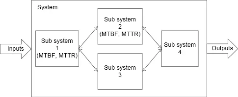
For reliability purposes, a system or product is decomposed into several components and reliability information is associated with these components. How do we determine these components? Many components can be extracted from the system architecture block diagram (Fig. 2.1). For hardware components, one natural division is to identify the Field Replaceable Units (FRU) and their reliability data estimates or measurements. FRUs are components, such as power supplies, fan trays, processors, memory, controllers, server blades, and routers, that can be replaced at the customer site by the customer or contracted field support staff. For software components, several factors need to be considered, such as system architecture, application layers, third party vendors, fault zones, and existing reliability information.

Figure 2.1 System Block Diagram

Let us say you have a system with several cages and lots of cards and have implemented fault tolerance mechanisms. If the design of the system is such that the customer's maintenance plan includes procedures for the repair of the system by replacing failed cards (FRUs), then at a minimum, those individual cards should be uniquely identified along with certain reliability data associated with them—in particular, MTBF and MTTR (Mean Time to Repair) data. This basic information is required to calculate system availability.

The MTTR is dependent upon how quickly a problem is identified and how quickly it can be repaired. In the telecom industry, typically a maintenance window exists at low traffic peak times of the day, during which maintenance activities take place. If a failed component does not affect the system significantly, then the repair of that component may be delayed until the maintenance window, depending on the customer's maintenance plan, ease of access to equipment, and so on. However, if the system functionality is significantly impacted due to a failure event, then the system will require immediate repair to recover full service.

In addition to hardware and software component failures, we should also take into consideration other possible failures and events that impact the availability of our system. These may include operator-initiated planned events (e.g., software upgrade), environment failures, security failures, external customer network failures, and operator errors. The objective is to identify those events and failures that can affect the ability of our system to provide full service, and create a model that incorporates these potential failures. We need to determine which of these events are significant (characterized by severity and likelihood of occurrence) and are within the scope of the system we are modeling. If we group certain failure modes into a fault zone, we can modularize the model for better analysis and maintainability.

2.3 Where Do We Get MTBF Information?

For hardware, we may be able to obtain MTBF information from industry standard data or from a manufacturer-published reliability data. If a particular component does not have a published or known MTBF, then the next step is to look for parts or components that are similar and estimate the MTBF based on that data under similar operating conditions. Another method is to extrapolate the MTBF based on data mining from past similar projects. In the worst case scenario, if a totally new component or technology is to be employed with little reliability data available, then a good rule of thumb is to look at a previous generation of products of a similar nature that do have some reliability data and use that information to estimate the MTBF. Use engineering judgment to decrease the MTBF by a reasonable factor, for example, x/2 to account for uncertainty and typical early failures in the hardware cycle. It is better to err on the side of caution.

Once we have made this initial assessment, the MTBF becomes the baseline for our initial model.

Let us consider a hypothetical communication system that consists of a chassis with several slots in which processing cards can be inserted. One of these cards is a new RF (radio frequency) carrier card. We start with the original data provided from the manufacturer, which indicate an MTBF of 550,000 hours. We then sanity-check these data by looking at MTBFs of similar cards successfully deployed over a number of years from different manufacturers. This analysis reveals an average MTBF of 75,000 hours. How might we reconcile the difference? Which estimate do we use? It turns out that the right answer may be both! In Chapter 13, we will explore techniques for combining reliability data to obtain an updated MTBF estimate that may be more accurate than any single source of MTBF data.

On the software side, if the software is being built in-house, we can derive the MTBF from similar projects that have been done in the past and at the same level of maturity. Release 1 always has the most bugs! We can also extrapolate information from field data in the current system release or previous releases. This can get more complicated if the software is written by multiple vendors (which is typical). We may also consider software complexity, risk, schedules, maturity of the organization developing the software, nonconstant failure rates, and so on as factors that affect MTBF.

Are you reusing existing software that has already been working in the field? For example, if we build on software from a previous project, and then we add additional functionality on top of this, we can extract software failure rate information from the previous project. We can also identify failure rates from industry information for common software, such as the Linux operating system. It is also quite possible that we identify MTBF information from third-party suppliers of off-the-shelf standard software.

We need to take into account as many relevant factors as possible when assigning MTBFs, MTTRs, and other reliability data. We should also note that MTBFs of products generally tend to improve over time—as the system gets more field exposure and software fixes are made, the MTBF numbers will generally increase.

2.4 MTTR and Identifying Failures

An important part of our architectural considerations is the detectability of the problem. How likely is it that when we have a problem, we will be able to automatically detect it? Fault Management includes designing detection mechanisms that are capable of picking up those failures.

Mechanisms, such as heartbeat messaging, checkpointing, process monitoring, checksums, and watchdog timers, help identify problems and potential failures. If a particular failure is automatically detected and isolated to a card, then recovery mechanisms can be invoked, for example, failover to a standby card.

Autorecovery is a useful technique for transient software failures, such as buffer overflows, memory leaks, locks that have not been released, and unstable or absorbing states that cause the system to hang. For these failures, a reboot of the card in which the problem was detected may repair the problem. If the failure reoccurs, more sophisticated repair actions may need to be employed. The bottom line is that we want to maximize the time the system is available leveraging the simplest recovery options for providing the required service.

In addition to detectable failures, a portion of the failures will be undetected or “silent” failures that should be accounted for as part of reliability calculations. These undetected failures can eventually manifest themselves as an impact to the functionality of the system. Since these failures may remain undetected by the system, the last line of defense is manual detection and resolution of the problem. Our goal is to reduce the number of undetected failures to an absolute minimum since these undetected failures potentially have a much larger impact on system functionality due to the length of time the problem remains undiscovered and uncorrected.

In situations where the problem cannot be recovered by an automatic card reset, for example, the MTTR becomes much larger. Instead of an MTTR of a few minutes to account for the reboot of a card, the MTTR could be on the order of several hours if we need to manually replace the card or system, or revert to a previous software version. So the more robust the system and fault management architecture is, the more successfully we can quickly identify and repair a failure. This is part of controllability—once we know the nature of the problem, we know the method that can be employed to recover from the problem.

There are several ways to reduce the MTTR. In situations where the software fails and is not responsive to external commands, we look at independent paths to increase the chances of recovering that card. In ATCA (Advanced Telecommunications Computing Architecture) architectures, a dedicated hardware line can trigger a reboot independent of the software. Other methods include internal watchdog time-outs that will trigger a card reboot. The more repair actions we have built into the system, the more robust it becomes. There is of course a trade-off on th...

Table of contents

• Cover
• IEEE Press
• Title page
• Copyright page
• Dedication
• Preface
• List of Abbreviations
• Chapter 1: Introduction
• Chapter 2: Initial Considerations for Reliability Design
• Chapter 3: A Game of Dice: An Introduction to Probability
• Chapter 4: Discrete Random Variables
• Chapter 5: Continuous Random Variables
• Chapter 6: Random Processes
• Chapter 7: Modeling and Reliability Basics
• Chapter 8: Discrete-Time Markov Analysis
• Chapter 9: Continuous-Time Markov Systems
• Chapter 10: Markov Analysis: Nonrepairable Systems
• Chapter 11: Markov Analysis: Repairable Systems
• Chapter 12: Analyzing Confidence Levels
• Chapter 13: Estimating Reliability Parameters
• Chapter 14: Six Sigma Tools for Predictive Engineering
• Chapter 15: Design Failure Modes and Effects Analysis
• Chapter 16: Fault Tree Analysis
• Chapter 17: Monte Carlo Simulation Models
• Chapter 18: Updating Reliability Estimates: Case Study
• Chapter 19: Fault Management Architectures
• Chapter 20: Application of DFMEA to Real-Life Example
• Chapter 21: Application of FTA to Real-Life Example
• Chapter 22: Complex High Availability System Analysis
• References
• Index