Fault Trees

Nikolaos Limnios

• Éditeur: Wiley-ISTE
• Année: 2013
• ISBN:
  9781118614068
• Édition: 1
• Sujet: Tecnología e ingeniería
• Sous-sujet: Ingeniería eléctrica y telecomunicaciones

Fault tree analysis is an important technique in determining the safety and dependability of complex systems. Fault trees are used as a major tool in the study of system safety as well as in reliability and availability studies.
The basic methods – construction, logical analysis, probability evaluation and influence study – are described in this book. The following extensions of fault trees, non-coherent fault trees, fault trees with delay and multi-performance fault trees, are also explained. Traditional algorithms for fault tree analysis are presented, as well as more recent algorithms based on binary decision diagrams (BDD).

Chapter 1

Single-Component Systems

1.1 Distribution of failure and reliability

1.1.1 Function of distribution and density of failure

We will study here the stochastic behaviour of single-component systems being subjected to failures (breakdowns) by observing them over a period of time. Let us simplify things by assuming that the system is put to work at the instant t = 0 for the first time and that it presents a single mode of failure.

The component, starting a lifetime period at the instant t = 0, is functioning for a certain period of time X₁ (random) at the end of which it breaks down. It remains in this state for a period of time Y₁ (random) during its replacement (or repair) and, at the end of this time, the component is again put to work and so on. In this case, the system is said to be repairable. In the contrary case, that is to say, when the component breaks down and continues to remain in this state, the system is said to be non-repairable.

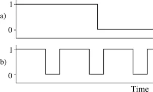
It is possible to present a graphic description of the behavior of the above- described system in different ways, the phase diagram being the most common.

Let X be a random variable (r.v.) representing the lifetime of the system with F, its cumulative distribution function (c.d.f.):

Figure 1.1 Phase diagrams: (a) non-repairable system and (b) repairable system 1: state of good functioning 0: state of breakdown

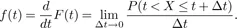
If F is absolutely continuous, the random variable X has a probability density function (p.d.f.) f and can be written as:

Regarding the probability evaluation of fault trees, we always have to make the distinction between the occurrence or arrival of an event and its existence at the time t. Let us consider, for example, that the f.r. F of the duration of life of a component has an p.d.f. f. The assertion “the occurrence of the failure of the component at the time t” means that the failure took place within the time interval (t, t +

t], where Δt → 0; as a result, its probability is given by: f(t)

t + o(

t). On the other hand, the assertion “existence of the failure at the time t” means that the failure took place at the time x ≤ t and its probab...

Table des matières

• Cover
• Titlepage
• Copyright
• Introduction
• Chapter 1: Single-Component Systems
• Chapter 2: Multi-Component Systems
• Chapter 3: Construction of Fault Trees
• Chapter 4: Minimal Sets
• Chapter 5: Probabilistic Assessment
• Chapter 6: Influence Assessment
• Chapter 7: Modules – Phases – Common Modes
• Chapter 8: Extensions: Non-Coherent, Delay and Multistate Fault Trees
• Chapter 9: Binary Decision Diagrams
• Chapter 10: Stochastic Simulation of Fault Trees
• Exercises
• Appendices
• Main Notations
• Bibliography
• Index