Representation of Complex Numbers

11 Key excerpts on "Representation of Complex Numbers"

• 

  eBook - PDF

  Mathematics NQF3 SB

  TVET FIRST

  • M Van Rensburg, I Mapaling, M Trollope A Thorne(Authors)
  • 2017(Publication Date)
  • Macmillan

    (Publisher)

  1 Module 1 Topic 1: Complex numbers Representing complex numbers in a form appropriate to the context Module 1 Learning Outcomes This module will show you how to do the following: • Unit 1.1: Write imaginary numbers in i -notation. • Unit 1.2: Simplify and perform addition, subtraction, multiplication and division on single-term imaginary numbers. • Unit 1.3: Construct Argand diagrams to find and represent complex numbers in standard/ rectangular form. • Unit 1.4: Represent complex numbers in polar form with modulus and positive argument. Figure 1.1: Sunglasses are created using the principles of imaginary and complex numbers. Figure 1.2: This small colour CCD spy camera is about 2 cm high and the electronic state in the materials is described by complex numbers. Figure 1.3: Mandelbrot fractals are created on a computer using complex numbers. Unit 1.1: Writing imaginary numbers in i -notation Pre-knowledge Figure 1.4: A graphical (visual) representation of the number system including complex numbers Real numbers ( ℝ ) Rational numbers ( ℚ ) Integers ( ℤ ) Whole numbers ( ℕ 0 ) Natural numbers ( ℕ ) Irrational numbers ( ℚ′ ) 4 __ 5 8 __ 9 0,2 1 2 3 4 5 − 6 − 8 − 1 − 4 ___ 7 √ __ 2 √ __ 3 √ __ 5 π Complex numbers z = 2 + 3 i 2 Module 1 Table 1.1: Revision of the different types of numbers Type Explanation Example Natural numbers ( ℕ ) All positive numbers used for counting and can be represented by the number line. ℕ = { 1; 2; 3; 4; 5; 6; 7; … } 1 2 3 4 5 6 7 Figure 1.5: Number line for natural numbers Whole numbers ( ℕ 0 ) All natural numbers including zero ℕ 0 = { 0; 1; 2; 3; 4; 5; 6; 7; … } Integers ( ℤ ) Positive and negative numbers (excluding decimals) ℤ = { …; − 3; − 2; − 1; 0; 1; 2; 3; … } Rational numbers ( ℚ ) Any number that can be written as a ratio hence the name rational. It can be written as a common fraction in the form: a __ b ; b ≠ 0. These include whole numbers, terminating decimals and non-terminating recurring decimals.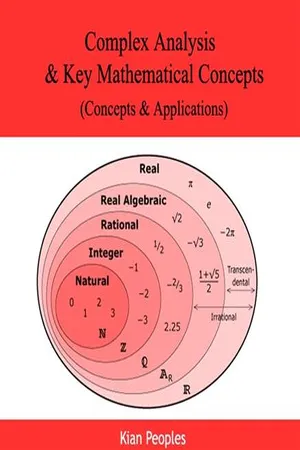

  Sign up to read

  Learn more about book
• 

  No longer available |Learn more

  Complex Analysis & Key Mathematical Concepts (Concepts & Applications)

  • (Author)
  • 2014(Publication Date)
  • Orange Apple

    (Publisher)

  A more abstract formalism for the complex numbers was further developed by the Irish mathematician William Rowan Hamilton, who extended this abstraction to the theory of quaternions. ________________________ WORLD TECHNOLOGIES ________________________ Complex numbers are used in a number of fields, including: engineering, electromagnetism, quantum physics, applied mathematics, and chaos theory. When the underlying field of numbers for a mathematical construct is the field of complex numbers, the name usually reflects that fact. Examples are complex analysis, complex matrix, complex polynomial, and complex Lie algebra. Complex numbers are plotted on the complex plane, on which the real part is on the horizontal axis, and the imaginary part on the vertical axis. Introduction and definition Complex numbers have been introduced to allow for solutions of certain equations that have no real solution: the equation x 2 + 1 = 0 has no real solution x , since the square of x is 0 or positive, so x 2 + 1 can not be zero. Complex numbers are a solution to this dilemma. The idea is to enhance the real numbers by adding a number i whose square is −1, so that x = i is a solution to the preceding equation. Definition A complex number is an expression of the form Here a and b are real numbers, and i is a mathematical symbol which is called imaginary unit . For example, -3.5 + 2 i is a complex number. The real number a of the complex number z = a + bi is called the real part of z and the real number b is the imaginary part .. They are denoted Re( z ) or ℜ ( z ) and Im( z ) or ℑ ( z ), respectively. For example, Some authors also write a + ib instead of a + bi . In some disciplines (in particular, electrical engineering, where i is a symbol for current), the imaginary unit i is instead written as j , so complex numbers are sometimes written as a + bj or a + jb .

  Sign up to read

  Learn more about book
• 

  eBook - PDF

  Complex Analysis

  • Donald E. Marshall(Author)
  • 2019(Publication Date)
  • Cambridge University Press

    (Publisher)

  PART I 1 Preliminaries 1.1 Complex Numbers The complex numbers C consist of pairs of real numbers: {(x, y) : x, y ∈ R}. The complex number (x, y) can be represented geometrically as a point in the plane R 2 , or viewed as a vector whose tip has coordinates (x, y) and whose tail has coordinates (0, 0). The complex number (x, y) can be identified with another pair of real numbers (r, θ ), called the polar coordinate representation. The line from (0, 0) to (x, y) has length r and forms an angle θ with the positive x axis. The angle is measured by using the distance along the corresponding arc of the circle of radius 1 (centered at (0, 0)). By similarity, the length of the subtended arc on the circle of radius r is rθ . See Figure 1.1. Conversion between these two representations is given by x = r cos θ , y = r sin θ and r =  x 2 + y 2 , tan θ = y x . Care must be taken to find θ from the last equality since many angles can have the same tan- gent. However, consideration of the quadrant containing (x, y) will give a unique θ ∈ [0, 2π ), provided r > 0 (we do not define θ when r = 0). Addition of complex numbers is defined coordinatewise: (a, b) + (c, d) = (a + c, b + d), and can be visualized by vector addition. See Figure 1.2. Multiplication is given by (a, b) · (c, d) = (ac − bd, bc + ad) and can be visualized as follows. The points (0, 0), (1, 0), (a, b) form a triangle. Construct a similar triangle with corresponding points (0, 0), (c, d), (x, y). Then it is an exercise in high- θ rθ r 1 x y (x, y) Figure 1.1 Cartesian and polar representations of complex numbers. 4 Preliminaries (a, b) (c, d) (a + c, b + d) Figure 1.2 Addition. (1, 0) (0, 0) (c, d) (a, b) (a, b) · (c, d) Figure 1.3 Multiplication. school geometry to show that (x, y) = (a, b) · (c, d). By similarity, the length of the product is the product of the lengths and polar coordinate angles are added. See Figure 1.3. The real number t is identified with the complex number (t, 0).

  Sign up to read

  Learn more about book
• 

  eBook - PDF

  Functions of a Complex Variable

  • Hemant Kumar Pathak, Ravi Agarwal, Yeol Je Cho(Authors)
  • 2015(Publication Date)
  • Chapman and Hall/CRC

    (Publisher)

  In general, when we write arg z , we mean the principal value of the argu-ment of z . 1.4 Geometrical Representations of Complex Numbers Consider the complex number z = x + iy . By the definition, z = ( x, y ) . This form of z suggests that z can be represented by a point P , as shown in Fig. 1.1, whose coordinates are x and y with respect to two rectangular axes XOX 0 and Y OY 0 , usually called the real and imaginary axes , respectively. The complex number z is called the affix of the point ( x, y ) which represents it. 5 K. Weierstrass calls the modulus of x + iy as the absolute value of x + iy and writes it as | x + iy | . 8 Functions of a Complex Variable FIGURE 1.1 : Cartesian and polar representations of z in plane. 1.5 Modulus and Argument of Complex Numbers Thus, to each complex number z , there corresponds one and only one point in the xy -plane and, conversely, to each point in this plane, there exists one and only one complex number. Such a plane is called complex plane or Gaussian plane or Argand plane . The Representation of Complex Numbers thus afforded is often called the Argand diagram 6 . 1.5.1 Polar Forms of Complex Numbers From Fig. 1.1, it is evident that, if x = r cos θ, y = r sin θ , then r = p x 2 + y 2 = | x + iy | = | z | , θ = tan -1 ( x y ) . It follows that z = x + iy = r (cos θ + i sin θ ) = re iθ . It is called the polar form of the complex number z . Thus the polar coordinates of P are ( r, θ ), where r is the modulus and θ the argument of the complex number z . 6 Named after the French mathematician Jean Robert Argand(1768–1822), born in Geneva and later a librarian in Paris. His paper on the complex plane appeared in 1806; it had however previously been used by Gauss, in his Helmstedt dissertation, 1790 (Werke, III. pp. 20–23), who had discovered it in Oct. 1797 ( Math. Ann. LVII. p. 18); and C. Wessel had discussed it in a memoir presented to the Danish Academy in 1797 and published by that society in 1798–9.

  Sign up to read

  Learn more about book
• 

  eBook - PDF

  The Shape of Algebra in the Mirrors of Mathematics

  A Visual, Computer-Aided Exploration of Elementary Algebra and Beyond (With CD-ROM)

  • Gabriel Katz, Vladimir Nodelman;;;(Authors)
  • 2011(Publication Date)
  • WSPC

    (Publisher)

  The Complex Numbers 105 Fig. 3.10 Your next task is to give the curve C a new analytical description: find formulas (in the polar coordinates { r , θ }) for a complex number w ( t ) so that, as t varies, the point u * w ( t ) will trace C . 3.6.3 A Short Historical Note The concept of a number that squares to -1 took hold slowly. The set of square roots of negative numbers were at first referred to as imaginary numbers—imaginary but useful. Geronimo Cardano, an Italian mathematician, used the concept in a published method of solving the cubic polynomial equation (1545). But this method was viewed with some suspicion because it depended on “imaginary” numbers for the calculations. Chapter 8 is devoted to the Cardano method and its ramifications. Early in the history of mathematics negative numbers were also termed “imaginary”, but this label eventually faded. Now the term “imaginary” is used to describe the set of vectors on the y -axis. They are of the form bi where b can be any real number. The Shape of Algebra 106 Recall that any number z of the form a + bi has its real part a = Re( z ) and its imaginary part b = Im( z ). The interpretation of complex numbers as vectors (points) in the Cartesian plane appears in the paper of Caspar Wessel published in 1799 in the Proceedings of Copenhagen Academy. In 1806, Jean-Robert Argand published an essay on the same subject. His paper is now viewed as the standard reference for the theoretic foundations of the vectorial Representation of Complex Numbers. In 1831, this geometric representation was rediscovered and popularized by Carl Friedrich Gauss. With this ingenious interpretation, the mystery of the imaginary was gone. 3.6.4 Division, Conjugation and Absolute Value Each complex number has a conjugate complex number associated with it . The conjugate of a + bi is defined as a – bi . The conjugate of a complex number z is commonly denoted z In VisuMatica, the conjugate of z is denoted by “conj(z)”.

  Sign up to read

  Learn more about book
• 

  eBook - ePub

  Elements of the Theory of Functions

  • Konrad Knopp, Bagemihl, Frederick(Authors)
  • 2016(Publication Date)
  • Dover Publications

    (Publisher)

  23 then we can write

  and this representation is obviously fully unique. Finally, according to §8 ,

  and so

  Thus, our new number system contains numbers whose squares are real and negative;—and likewise, as it will turn out, all the remaining “impossibilities” mentioned in §4 have now turned into realities. In this sense, then, it constitutes a consistent extension of the system of real numbers, and, indeed, one which no longer possesses the deficiencies of the latter.

  Since every complex number a = (α, α′) can be represented in the form

  the operations with complex numbers can also be regarded as operations with sums of this form, in which α and α′ are real numbers, and i is a number symbol for which i2 , i.e., (0,1) · (0, 1), is equal to – 1.

  The same goal—the removal of the deficiencies of the system of real numbers by means of suitable extensions of the same, consistent with the fundamental laws—cannot be reached in any (essentially) different manner; but we shall not go into this.

  11. Trigonometric Representation of Complex Numbers

  In what precedes, we have used Cartesian coordinates to represent points and vectors. If we take polar coordinates, some things become simpler, others, less simple.

  If ρ and φ are the polar coordinates of the point a = (α, α′), then, according to §5 ,

  The number a = α + α′i can therefore be represented in the form

  This is called the trigonometric representation of a complex number. In antithesis to it, the representation a = α + α′i may be designated as the Cartesian. In the latter, the real and imaginary-parts are displayed; in the former, absolute value and amplitude. The last quantity appears only in the combination (cos φ + i sin φ); this factor is called the direction factor of the complex number a

  Sign up to read

  Learn more about book
• 

  eBook - PDF

  Guide to Mathematical Methods

  • John Gilbert, Camilla Jordan, David A Towers(Authors)
  • 2017(Publication Date)
  • Red Globe Press

    (Publisher)

  13.2 The algebra of complex numbers Complex numbers first appeared in the sixteenth century in the work of the Italian mathematician Bombelli. They arose in connection with the solutions of equations, cubic as well as quadratic, and appeared in the form x + i y (13.1) where x and y are real numbers and i is a ‘number’ whose square is − 1. The existence and nature of this ‘number’ i gave rise to a certain amount of mystery and scepticism, some of which lingers on through the use of the term ‘imaginary number’. We shall give a definition of a complex number which overcomes the problem of existence. In practice we think of complex numbers in the above form and we shall see how our definition is consistent with this. Definition 13.1 A complex number is an ordered pair ( x, y ) of real num-bers, usually written as x + i y . The use of the word ‘ordered’ in the definition is important; the ordered pairs ( x, y ) and ( y, x ) are distinct unless x = y . The set of all complex numbers is denoted by C and it is usual to denote a typical member of the set by the single letter z . This is often more convenient in manipulations than the fuller form x + i y . Complex numbers can be represented as points in the Cartesian plane in an obvious way: x + i y is represented by the point with Cartesian coordinates ( x, y ). For example, the number 2 − 3i (note that we write the second number, -3, in front of the i) is plotted as the point (2 , − 3). We usually refer to the plane as the Argand diagram in this context. Figure 13.1 shows an example, with the point 2 − 3i and other points marked on it. The complex number 334 Guide to Mathematical Methods − 4i − 3i − 2i − i i 2i 3i 4i − 4 − 3 − 2 − 1 1 2 1 4 R I 4 + i − 1 + 4i − 4 − 2i 2 − 3i Figure 13.1: Argand diagram 0 + 1i is usually written as i. If x is a real number then we write it in the form of a complex number as x + 0i. Thus, in the Argand diagram, real numbers appear on the x axis, sometimes called the real axis for this reason.

  Sign up to read

  Learn more about book
• 

  eBook - PDF

  Technical Mathematics with Calculus

  • Paul A. Calter, Michael A. Calter(Authors)
  • 2011(Publication Date)
  • Wiley

    (Publisher)

  Why another form? We will see that while addition and subtraction of complex numbers are best done in rectangular form, multiplication and division are easier in polar form. Figure 19–5 shows how the rectangular and polar forms are related. There we have plotted the complex number If we now connect that point to the origin by a line segment of length r, it makes an angle with the horizontal axis. We can express the same complex number in terms of r and , if we note that So Similarly, Substituting gives (1) We can also write this expression using the simpler notation, (2) A third polar form can be obtained from Euler’s formula, Eq. 185, which we give without proof. Here e is the base of natural logarithms and is in radians. Multiplying both sides by r, we get So, (3) While Eqs. 1, 2, and 3 are polar forms of a complex number, we will refer to Eq. 1 as the trigonometric form, Eq. 2 as the polar form, and Eq. 3 as the exponential form. In all three polar forms, r is called the magnitude or absolute value of the complex number, and the angle is called the argument of the complex number. u re iu a  bi  re iu r(cos u  i sin u)  u e iu cos u  i sin u  a  bi  r l u  r (cos u  i sin u) a  bi  r cos u  ri sin u b  r sin u a  r cos u cos u  a r u u a  bi. (9  3i)  (2  4i) (7i  2)  (3i  5) (5  6i)  (3  2i) (2  3i)  (1  i) 8  (4  i) (4  2i)  2 44i  2i 12i  6i 9  3i 8i  4 5  8i mi  n 5i  6 p  qi 5  7i 2  3i 0 a + bi = r  r  Imaginary Real a b FIGURE 19–5 Polar form of a complex number shown on a complex plane. Named for the Swiss mathematician Leonhard Euler (1707–1783). Section 2 ◆ Complex Numbers in Polar Form 569 Our various forms of a complex number are then 169 170 171 172 where 173 174 175 176 In practice, we will just use the rectangular form for addition and subtraction, and the polar form for multiplication and division. Converting between Rectangular and Polar Form To convert from rectangular to polar we use Eqs.

  Sign up to read

  Learn more about book
• 

  eBook - PDF

  Numbers and Proofs

  • Reg Allenby(Author)
  • 1997(Publication Date)
  • Butterworth-Heinemann

    (Publisher)

  We make the complex number a + ib correspond to the point whose (Cartesian) coordinates are (a, b). Thought of in this way, the real plane is sometimes called the Argand diagram. However, the plane can be coordinatized in many ways, one of which is by using polar coordinates. A diagram should help. From Figure 10.1 we see that, if a point has Cartesian coordinates (x,y) and polar coordinates (r, £)), then x = r cos $ and y = r sin 5. It is easily checked that r = + yj{x 2 + y 2 ) whilst if θ is chosen so that — π < θ ^ π then $ is one of the two possible angles for which tan 9 = y/x. Hence if a is the complex number x + iy then a = r(cosi9 + isinS). This is called the polar form of a. The value r is called the THE REAL NUMBERS AND THE COMPLEX NUMBERS 165 y b 0 r / ^ θ^ (a,t a x Figure 10.1 modulus of a and we write r = |a|. As drawn, — π < $ ^ π and as such 5 is called the principal argument or principal amplitude of a, written S = Arg(a) with a capital Ά'. However, since, for all integers n, and cos (S + 2ηπ) = cos $ sin (5 + 2rar) = sin$ it is often convenient to regard any one (or indeed all) of these angles 9 + 2ηπ as an argument (or amplitude) of a. We then write 9 = arg(a) - using a small 'a'. The expression r(cos# + isin$) is often abbreviated to rcis$. EXERCISE 8 For each of the following complex numbers a, find the modulus |a| and the principal value Arg(a) of the argument. Then write a in polar form: (a) 2 (b) -3 (c) cos 9 + i sin $ (d) cos $ — i sin 9 (e) i (f) -i (g) 1 + i (h) 1 - i (i) 3 -4 i (j) 11 + 60Í (k) sin73° + icos73° EXERCISE 9 Write the following complex numbers in Cartesian form: (a) cisf; (b) cis^; (c) 4cisn; (d) v^cisf.

  Sign up to read

  Learn more about book
• 

  eBook - PDF

  Technical Mathematics with Calculus

  • Michael A. Calter, Paul A. Calter, Paul Wraight, Sarah White(Authors)
  • 2016(Publication Date)
  • Wiley

    (Publisher)

  21 ◆◆◆ OBJECTIVES ◆◆◆◆◆◆◆◆◆◆◆◆◆◆◆◆◆◆◆◆◆◆◆◆◆◆◆◆◆◆◆◆◆◆◆◆◆◆◆◆◆◆◆◆◆◆◆◆◆◆◆◆◆◆◆◆◆◆◆ When you have completed this chapter, you should be able to: • Identify the characteristics of imaginary and complex numbers. • Graph complex numbers. • Express complex numbers in trigonometric and polar form. • Express complex numbers in exponential form. • Represent vectors using complex numbers. • Apply the characteristics of complex numbers and solve alternating-current problems. Complex numbers—a poor name for this mathematical technique, as they are actually very straightforward. A complex number is used as a coordinate on a two-dimensional plane, almost exactly like an x, y coordinate. The difference is that the x axis is the real number line and the y axis is the imaginary number line. Complex numbers allow you to work much more easily with vectors. Mathematicians developed this imaginary number line to solve the mathematical problem of finding the square root of a negative number. The square root of any negative number is not solvable by a real number because there are no two identical roots that when multiplied together will give you a negative number. However, if you multiply a positive number, say 3, by the square root of -1 twice, you get 0 –1 –2 –3 –4 +1 +2 +3 +4 3 1 1 3 1 3 × - × - = × - = - FIGURE 21-1 And if you multiply a negative number, say -2, by the square root of -1 twice, you get 2 1 1 2 1 2 - × - × - = - × - = 0 –1 –2 –3 –4 +1 +2 +3 +4 FIGURE 21-2 Even if we can’t write an actual number value for 1 - , we see that the effect of multiplying a number by the square root of -1 twice is like rotating 180° onto the opposite side of the num- ber line. From +3 to -3 (Fig. 21-1) or from -2 to +2 (Fig. 21-2), it seems that we are not so much multiplying by a number as rotating about the zero of the number line. So, if multiply- ing twice is a 180° rotation, multiplying once must be a 90° rotation. But a rotation to where? Complex Numbers

  Sign up to read

  Learn more about book
• 

  eBook - PDF

  Quantum Computing for Computer Scientists

  • Noson S. Yanofsky, Mirco A. Mannucci(Authors)
  • 2008(Publication Date)
  • Cambridge University Press

    (Publisher)

  These fellows, being akin to i , are known as imaginary numbers. But there is more: add a real number and an imaginary number, for instance, 3 + 5 × i , and you get a number that is neither a real nor an imaginary. Such a number, being a hybrid entity, is rightfully called a complex number. Definition 1.1.1 A complex number is an expression c = a + b × i = a + bi , (1.5) where a, b are two real numbers; a is called the real part of c, whereas b is its imaginary part. The set of all complex numbers will be denoted as C. When the × is understood, we shall omit it. Complex numbers can be added and multiplied, as shown next. Example 1.1.2 Let c 1 = 3 − i and c 2 = 1 + 4i . We want to compute c 1 + c 2 and c 1 × c 2 . c 1 + c 2 = 3 − i + 1 + 4i = (3 + 1) + (−1 + 4)i = 4 + 3i . (1.6) Multiplying is not as easy. We must remember to multiply each term of the first complex number with each term of the second complex number. Also, remember that i 2 = −1. c 1 × c 2 = (3 − i ) × (1 + 4i ) = (3 × 1) + (3 × 4i ) + (−i × 1) + (−i × 4i ) = (3 + 4) + (−1 + 12)i = 7 + 11i . (1.7)  Exercise 1.1.3 Let c 1 = −3 + i and c 2 = 2 − 4i . Calculate c 1 + c 2 and c 1 × c 2 .  With addition and multiplication we can get all polynomials. We set out to find a solution for Equation (1.1); it turns out that complex numbers are enough to provide solutions for all polynomial equations. Proposition 1.1.1 (Fundamental Theorem of Algebra). Every polynomial equa- tion of one variable with complex coefficients has a complex solution. Exercise 1.1.4 Verify that the complex number −1 + i is a solution for the polyno- mial equation x 2 + 2x + 2 = 0.  This nontrivial result shows that complex numbers are well worth our attention. In the next two sections, we explore the complex kingdom a little further. Programming Drill 1.1.1 Write a program that accepts two complex numbers and outputs their sum and their product.

  Sign up to read

  Learn more about book