Mathematics
Standard Normal Distribution
The standard normal distribution is a probability distribution that has a mean of zero and a standard deviation of one. It is a bell-shaped curve that is symmetric around the mean and is widely used in statistical analysis to model random variables that have a normal distribution.
Written by Perlego with AI-assistance
Related key terms
1 of 5
12 Key excerpts on "Standard Normal Distribution"

- Harold O. Kiess, Bonnie A. Green(Authors)
- 2019(Publication Date)
- Cambridge University Press(Publisher)
Normal distribution 3 A theoretical mathematical distribution that specifies the relative frequency of a set of scores in a population. mean ( ) and the standard deviation ( ) of the distribution. A normal distribution with and is illustrated in Figure 6.1. The distribution shown is a mathemati- cal distribution that does not represent any actually measured population of scores. No real population of scores is distributed so precisely that it will be exactly normal, but it will be useful at times to assume that some populations of scores are approximately nor- mally distributed. In this chapter, however, we focus on the normal distribution as a the- oretical mathematical distribution. The Normal Distribution and the Behavioral Sciences The normal distribution developed from the work of Jakob Bernoulli (1654–1705), Abraham de Moivre (1667–1754), Pierre Remond de Montmort (1678–1719), Karl Friedrich Gauss (1777–1855), and others. Their interests were in developing mathematical approximations for probabilities encountered in various games of chance or in the distribution of errors to be expected in observations, such as in astronomy or physics. The normal distribution soon became an important distribution to statisticians because many problems in statistics can be solved only if a normal distribution is assumed. = 10 = 70 CHAPTER 6 The Normal Distribution, Probability, and Standard Scores 107 6.1 TABLE Notation for samples and populations Sample Population Descriptive characteristics Statistics Parameters Mean Standard deviation s Variance s 2 2 X .40 .30 .20 .10 Relative frequency 100 + 3 90 + 2 80 + 1 70 60 – 1 50 – 2 40 – 3 Scores .00 Figure 6.1 A normal distribution with and . = 10 = 70 The normal distribution also gained importance for behavioral scientists because it is reasonable to assume that any behavioral measures determined by a large number of inde- pendent variables will be approximately normally distributed for a population.
- James E. De Muth(Author)
- 2014(Publication Date)
- Chapman and Hall/CRC(Publisher)
99 6 The Normal Distribution and Data Transformation Described as a “bell-shaped” curve, the normal distribution is a symmetrical distribution that is one of the most commonly occurring outcomes in nature and its presence is assumed in several of the most commonly used statistical tests. Properties of the normal distribution have a very important role in the statistical theory of drawing inferences about population parameters (estimating confidence intervals) based on samples drawn from that population. There are ways to transform initial data to produce distributions approximating a normal distribution. Various graphic and mathematical methods are available to test for normality. The Normal Distribution The normal distribution is the most important distribution in statistics. This curve is a special frequency distribution that describes the population distribution of many continuously distributed biological traits. The normal distribution is often referred to as the Gaussian distribution , after the mathematician Carl Friedrich Gauss, even though a formula to calculate a normal distribution was first reported by the French mathematician Abraham DeMoivre in the mid-eighteenth century (Porter, 1986). It is critical at this point to realize that we are focusing our initial discussion on the total population, not a sample . As mentioned in the previous chapter, in the population, the mean is expressed as μ and standard deviation as σ . Sample data ( X and S ) are the best estimates of these population parameters and the distribution of the Mean Chapter 6 100 Figure 6.1 Proportions between various standard deviations under a normal distribution. sample data provides the best estimator of the population distribution. The characteristics of a normal distribution are as follows. First, the normal distribution is continuous and the curve is symmetrical about the mean. Second, the mode, median, and mean are equal and represent the middle of the distribution.
- Brase/Brase, Charles Henry Brase, Corrinne Pellillo Brase(Authors)
- 2016(Publication Date)
- Cengage Learning EMEA(Publisher)
The Standard Normal Distribution is a normal distribution with mean m 5 0 and standard deviation s 5 1 (Figure 7-12). Standard Normal Distribution Any normal distribution of x values can be converted to the Standard Normal Distribution by converting all x values to their corresponding z values. The resulting standard distribution will always have mean m 5 0 and standard deviation s 5 1 . FIGURE 7-12 The Standard Normal Distribution 1 m 5 0, s 5 1 2 WHAT DOES THE Standard Normal Distribution TELL US? When we have the Standard Normal Distribution, we know • the mean is 0. • the standard deviation is 1. • any normal distribution can be converted to a standard normal dis -tribution by converting all the measurements to standard z scores. AREAS UNDER THE STANDARD NORMAL CURVE We have seen how to convert any normal distribution to the standard normal dis-tribution. We can change any x value to a z value and back again. But what is the advantage of all this work? The advantage is that there are extensive tables that show the area under the standard normal curve for almost any interval along the z axis. The areas are important because each area is equal to the probability that the measurement of an item selected at random falls in this interval. Thus, the Standard Normal Distribution can be a tremendously helpful tool. USING A Standard Normal Distribution TABLE Using a table to find areas and probabilities associated with the standard normal dis-tribution is a fairly straightforward activity. However, it is important to first observe Area under the standard normal curve © Cengage Learning ® Copyright 2017 Cengage Learning. All Rights Reserved. May not be copied, scanned, or duplicated, in whole or in part. Due to electronic rights, some third party content may be suppressed from the eBook and/or eChapter(s). Editorial review has deemed that any suppressed content does not materially affect the overall learning experience. eBook - PDF
- Roy E Bruns, Ieda Spacino Scarminio, Benicio de Barros Neto(Authors)
- 2006(Publication Date)
- Elsevier Science(Publisher)
If we could discover or estimate the nature of this distribution, we could calculate the probability of occurrence of any value of interest. We would, in fact, possess a sort of statistical crystal ball we could use to make predictions. Soon we will see how to do this using the normal distribution. The normal distribution is a continuous distribution, that is, a distribution in which the variable can assume any value within a predefined interval. For a normally distributed variable, this interval is ( N , + N ), which means that the variable can — in principle — assume any real value. A continuous distribution of the variable x is defined by its probability density function f ( x ), a mathematical expression containing a certain number of parameters. The normal distribution is fully defined by two parameters, its mean and its variance (Eq. (2.5)). The normal distribution: f ð x Þ d x ¼ 1 s ffiffiffiffiffi 2 p p e x m ð Þ 2 = 2 s 2 d x (2.5) f ð x Þ ¼ probability density function of the random variable x ; m ¼ population mean; s 2 ¼ population variance. 13 Although Gauss is the mathematician most commonly associated with the normal distribution, the history behind it is more involved. At least Laplace, De Moivre and one of the ubiquitous Bernoullis seem to have worked on it too. Chapter 2 24 To indicate that a random variable x is normally distributed with mean m and variance s 2 ; we use the notation x N ð m ; s 2 Þ ; where the notation stands for ‘‘is distributed in accordance with’’. If x has zero mean and unit variance, for example, we write x N ð 0 ; 1 Þ and say that x follows the standard (or unit ) normal distribution. Fig. 2.3 shows the famous bell-shaped curve that is the plot of the probability density of the Standard Normal Distribution, f ð x Þ ¼ 1 ffiffiffiffiffi 2 p p e x 2 = 2 . (2.5a) Note that the curve is perfectly symmetrical about its central point, the mean m (here equal to zero).
- David Howell(Author)
- 2020(Publication Date)
- Cengage Learning EMEA(Publisher)
The normal distribution is a very common distribution in statistics, and it is often taken as a good description of how observations on a dependent variable are distributed. We very often assumed that the data in our sample came from a normally distributed population. This chapter began by looking at a pie chart representing people under correc-tional supervision. We saw that the area of a section of the pie is directly related to the probability that an individual would fall in that category. We then moved from the pie chart to a bar graph, which is a better way of presenting the data, and then moved to a histogram of data that have a roughly normal distribution. The purpose of those transitions was to highlight the fact that area under a curve can be linked to probability. The normal distribution is a symmetric distribution with its mode at the cen-ter. In fact, the mode, median, and mean will be the same for a variable that is nor-mally distributed. We saw that we can convert raw scores on a normal distribution to z scores by simply dividing the deviation of the raw score from the population mean ( m ) by the standard deviation of the population ( s ). The z score is an important statistic because it allows us to use tables of the Standard Normal Distribution (often denoted N ( m , s 2 )). Once we convert a raw score to a z score we can immediately use the tables of the Standard Normal Distribution to compute the probability that any observation will fall within a given interval. We also saw that there are a number of measures that are directly related to z . For example, data are often reported as coming from a population with a mean of 50 and a standard deviation of 10. eBook - PDF
- Barbara Illowsky, Susan Dean(Authors)
- 2020(Publication Date)
- Openstax(Publisher)
The z-score allows us to compare data that are normally distributed but scaled differently. CHAPTER REVIEW 6.1 The Standard Normal Distribution A z-score is a standardized value. Its distribution is the standard normal, Z ~ N(0, 1). The mean of the z-scores is zero and the standard deviation is one. If z is the z-score for a value x from the normal distribution N(µ, σ), then z tells you how many standard deviations x is above—greater than—or below—less than—µ. 6.2 Using the Normal Distribution The normal distribution, which is continuous, is the most important of all the probability distributions. Its graph is bell- shaped. This bell-shaped curve is used in almost all disciplines. Since it is a continuous distribution, the total area under the curve is one. The parameters of the normal are the mean µ and the standard deviation σ. A special normal distribution, called the Standard Normal Distribution, is the distribution of z-scores. Its mean is zero, and its standard deviation is one. FORMULA REVIEW 6.0 Introduction X ∼ N(μ, σ) μ = the mean, σ = the standard deviation 6.1 The Standard Normal Distribution Z ~ N(0, 1) z = a standardized value (z-score) mean = 0, standard deviation = 1 To find the k th percentile of X when the z-score is known, k = μ + (z)σ z-score: z = x – μ σ Z = the random variable for z-scores 6.2 Using the Normal Distribution Normal Distribution: X ~ N(µ, σ), where µ is the mean and σ is the standard deviation Standard Normal Distribution: Z ~ N(0, 1). Calculator function for probability: normalcdf (lower x value of the area, upper x value of the area, mean, standard deviation) Calculator function for the k th percentile: k = invNorm (area to the left of k, mean, standard deviation) PRACTICE 6.1 The Standard Normal Distribution 1. A bottle of water contains 12.05 fluid ounces with a standard deviation of 0.01 ounces. Define the random variable X in words. X = ____________. 2. A normal distribution has a mean of 61 and a standard deviation of 15. No longer available |Learn more
- Anthony Hayter(Author)
- 2012(Publication Date)
- Cengage Learning EMEA(Publisher)
C H A P T E R F I V E The Normal Distribution In this chapter the normal or Gaussian distribution is discussed. It is the most important of all continuous probability distributions and is used extensively as the basis for many statistical inference methods. Its importance stems from the fact that it is a natural probability distribution for directly modeling error distributions and many other naturally occurring phenomena. In addition, by virtue of the central limit theorem , which is discussed in Section 5.3, the normal distribution provides a useful, simple, and accurate approximation to the distribution of general sample averages. 5.1 Probability Calculations Using the Normal Distribution 5.1.1 Definition of the Normal Distribution The Normal Distribution The normal or Gaussian distribution has a probability density function f ( x ) = 1 σ √ 2 π e − ( x − μ) 2 / 2 σ 2 for −∞ ≤ x ≤ ∞ , depending upon two parameters, the mean and the variance E ( X ) = μ and Var ( X ) = σ 2 of the distribution. The probability density function is a bell-shaped curve that is symmetric about μ . The notation X ∼ N (μ, σ 2 ) denotes that the random variable X has a normal distribution with mean μ and variance σ 2 . In addition, the random variable X can be referred to as being “normally distributed.” HISTORICAL NOTE Carl Friedrich Gauss (1777–1855) ranks as one of the greatest mathematicians of all time. He studied mathematics at the University of G¨ ottingen, Germany, between 1795 and 1798 and later in 1807 became professor of astronomy at the same university, where he remained until his death. His work on the normal distribution was performed around 1820. He is reported to have been deeply religious, aristocratic, and conservative. He did not enjoy teaching and consequently had only a few students. The probability density function of a normal random variable is symmetric about the mean value μ and has what is known as a “bell-shaped” curve. eBook - PDF
Statistics
Principles and Methods
- Richard A. Johnson, Gouri K. Bhattacharyya(Authors)
- 2019(Publication Date)
- Wiley(Publisher)
It can be symmetric about the mean of X or it can be skewed, meaning that it has a long tail to either the left or the right. The probability that X lies in an interval from a to b is determined by the area under the probability density curve between a and b. The total area under the curve is 1, and the curve is never negative. The population 100 p-th percentile is an x value that has probability p to its left and probability 1 − p to its right. When X has mean and standard deviation , the standardized variable Z = X − has mean 0 and standard deviation 1. The normal distribution has a symmetric bell-shaped curve centered at the mean. The intervals extending one, two, and three standard deviations around the mean contain the probabilities .683, .954, and .997, respectively. If X is normally distributed with mean and standard deviation , then Z = X − has the Standard Normal Distribution. When the number of trials n is large and the success probability p is not too near 0 or 1, the binomial distribution is well approximated by a normal distribution with mean n p and sd = √ n p ( 1 − p ). Specifically, the probabilities for a binomial variable X can be approximately cal- culated by treating Z = X − n p √ n p ( 1 − p ) as standard normal. For a moderate number of trials n, the approximation is improved by appro- priately adjusting by 1 2 called a continuity correction. 206 CHAPTER 6/THE NORMAL DISTRIBUTION The normal scores are an ideal sample from a Standard Normal Distribution. Plotting each ordered observation versus the corresponding normal score creates a normal-scores plot, which provides a visual check for possible departures from a normal distribution. Transformation of the measurement scale often helps to convert a long-tailed distribution to one that resembles a normal distribution. eBook - PDF
Comparative Analysis Of Nations
Quantitative Approaches
- Robert Perry(Author)
- 2019(Publication Date)
- Routledge(Publisher)
Unfortunately, as any student of cross-national analysis is all too painfully aware, data availability and the sheer limitation of the number of countries within the world make 94 The Role if the Normal Distribution in Cross-National Research 95 samples that perfectly conform to assumptions of the normal distribution a rarity (if not an impossibility). This, however, should not preclude students from becoming fa-miliar with the uncomfortable, and often challenging, task of thinking beyond the properties of the literal sample to considering the more abstract, and practical, impli-cations that are inherent within the statistical analysis of their samples. In this chapter we will introduce you to a more detailed discussion of the logic of the normal distribution, with particular reference to the standard areas under the nor-mal curve. Once you have grasped the logic of the normal distribution, we can then show how to use the statistical output from univariate analysis to formulate assess-ments of the population's general properties and to go from there to a consideration of country-specific comparisons. The workhorse statistics in this chapter are once again the mean and standard deviation. Our goal, in this chapter and the next, is to apply the mean and standard deviation, not merely interpret their meaning. In applying these two statistics we often rely upon the construction of a critical statistic called the z-score. We will show how one com-putes and interprets a z-score, and how it plays an indispensable role in cross-national analysis. While the beginning student often dismisses discussions of the normal distribution as boring and overly detailed, the truth is that the logic of the normal distribution of-fers the student of cross-national analysis important insight that is invaluable in the broader enterprise of comparison. eBook - PDF
Finite Mathematics
Models and Applications
- Carla C. Morris, Robert M. Stark(Authors)
- 2015(Publication Date)
- Wiley(Publisher)
Sometimes, the probabilities are given, as in a quality standard of, say, 95%, and other parameters are to be calculated. Actually, there are four relevant quanti- ties – probability, variable value, mean, and standard deviation. The above examples have used the last three to obtain probabilities. Actually, any three can be used to determine the fourth, as illustrated in the next examples. Example 10.4.9 The Standard Normal Random Variable Find a value of the standard normal random variable z, call it z 0 , such that a) P(z > z 0 ) = 0.7764 b) P(−z 0 < z < z 0 ) = 0.9500 c) P(−1.64 < z < z 0 ) = 0.1915 Solution: a) To determine z 0 such that P(z > z 0 ) = 0.7764, so the probability exceeds 1 ∕ 2 (figure below). Therefore, z 0 must be negative. There is a 0.2764 probability (0.7764 − 0.5000) between z 0 and 0. Looking for 0.2764 or its closest in the table interior, find the corresponding z score as 0.76. Here, z 0 = −0.76. z 0 0 0.2764 0.5000 f (z) b) To determine z 0 such that P(−z 0 < z < z 0 ) = 0.9500, first note the symmetry. Each side of the zero has the same probability, 0.9500 ∕ 2 = 0.4750. Reading from 0.4750 in the table interior (and working to the margin), we find z 0 = 1.96. There is a 95% probability that z lies between −1.96 and +1.96. –z 0 0 z 0 0.4750 0.4750 f (z) c) To determine z 0 such that P(−1.64 < z < z 0 ) = 0.1915, first determine the prob- ability for the known z-score. The probability that z 0 lies between −1.64 and 0 is 0.4495, as z 0 is negative. Regions a and b combined (figure) represent a total THE NORMAL DISTRIBUTION 345 probability of 0.4495. However, region a represents a probability of 0.1915, leaving region b to a probability of 0.2580. This probability, in the interior of the table, has z 0 as −0.70. As a check, P(−1.64 < z < −0.70) = 0.1915! –1.64 z 0 0 0.2580 0.1915 a b Example 10.4.10 Regulating Machine Settings For a normal distribution, the probability that x is less than 118 is to be 4 ∕ 5.
- Adam Prügel-Bennett(Author)
- 2020(Publication Date)
- Cambridge University Press(Publisher)
98 The Normal Distribution To check the normalisation of the normal distribution we change variables y = V ( x − μ), which gives ∞ −∞ N( x| μ, Σ) d x = 1 |2πΣ| ∞ −∞ e − y V T Σ −1 V y /2 J n i=1 dy i where J is the Jacobian defined by J = ∂x 1 ∂y 1 ∂x 1 ∂y 2 · · · ∂x 1 ∂yn ∂x 2 ∂y 1 ∂x 2 ∂y 2 · · · ∂x 2 ∂yn . . . . . . . . . . . . ∂xn ∂y 1 ∂xn ∂y 2 · · · ∂xn ∂yn . Since x = V T y + μ we find J = |V T |. The determinant of an orthogonal matrix is should be ±1. A matrix can be thought of as mapping points from one space to another space. If we map all points in some volume in the first space to the second space, then the ratio of volumes is given by the determinant (up to a sign describing whether that volume suffers a reflection or not). Because an orthogonal matrix just corresponds to a rotation and a possible reflection the determinant is ±1. Returning to the integral and using the diagonalisation formula we find ∞ −∞ N( x | μ, Σ) d x = 1 |2πΣ| ∞ −∞ e − y Λ −1 y /2 n i=1 dy i = 1 |2πΣ| n i=1 ∞ −∞ e −y 2 i /(2λ i ) dy i = 1 |2πΣ| n i=1 2 π λ i = (2 π) n/2 n i=1 λ i |2πΣ| . If M is an n × n matrix then |a M| = a n |M|. Thus the factors of 2 π cancel each other out. Using the property of the determinant |A B| = |A| × |B| (which immediately implies |A B C| = |A| × |B| × |C|), |Σ| = |VΛV T | = |V| × |Λ| × |V T | = |Λ|, since the determinants of the orthogonal matrix are equal to ±1. However, the determinant of a diagonal matrix is equal to the product of its diagonal elements so that |Λ| = n i=1 λ i , which completes our verification of the normalisation of the normal distribution. It follows from this derivation that if X ∼ N( μ, Σ) where Σ = VΛV T then Y = Λ −1/2 V( X − μ) will be distributed according to N(0, I). That is, the components of Y are independent normally distributed variables with zero mean and unit variance.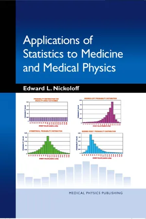
- Edward L. Nickoloff(Author)
- 2011(Publication Date)
- Medical Physics Publishing(Publisher)
Table 3.6 and illustration 3.6 give the integral values. The cumulative Normal probability for distances +/−R (where R is in units of σ) from the mean can be approximated by (3.17). R is calculated by the expression [(X i − μ)/σ]. Pr . exp x X i ( ) = ( ) ⎡ ⎣ ⎢ ⎢ ⎤ ⎦ ⎥ ⎥ − − ( ) ( ) ⎧ ⎨ ⎪ ⎩ ⎪ 1 0 2 2 2 2 σ π μ σ ⎫ ⎬ ⎪ ⎭ ⎪ ⎡ ⎣ ⎢ ⎢ ⎤ ⎦ ⎥ ⎥ . Illustration 3.5: One-Tailed Cumulative Probability Area from +X ′ 0 to +∞ (3.17) where a ≅ 0.63 and R = (X i − m)/s. For 0.1 < R < 3.0, the approximation given above is accurate to within +/− a few percent for a two-tailed cumulative Normal distribution about the mean value. Thus, the concept of standard deviation defines the statistical dispersion (or spread) in the measured values. Cumulative Probability R ≈ − − ( ) { } ⎡ ⎣ ⎤ ⎦ 1 0 2 0 . exp . α 5 , More Details about the Normal Probability Distributions ■ 63 Table 3.6: Integral values for the Normal function The key item to remember is that 68.3% of all measurements are within ±1 σ of the mean value. 95.5% of all measurements are within ±2 σ of the mean values. Nearly all the measurements (99.7%) are within ±3 σ of the mean value. 64 ■ Chapter 3 3.10 CONFIDENCE INTERVALS Confidence intervals are sometimes called “fences.” They delineate the range of values over which any set of data is expected to be dispersed. The intervals are based upon the cumulative value of the Normal probability distribution. The most common confidence intervals are “Two-Tailed”; i.e., with a certain level of confidence expressed as a percentage, the data are expected to be within the range “mean ± ε.” The ε range is based upon the number of standard deviations from the mean value, and the confidence level is based upon the cumulative probability value for that number of standard deviations. For example, the data are expected to be within “mean − 2σ” to “mean + 2σ” with 95.5% confidence level. Commonly used con- fidence values are 90%, 95%, 98%, and 99%.
Index pages curate the most relevant extracts from our library of academic textbooks. They’ve been created using an in-house natural language model (NLM), each adding context and meaning to key research topics.