Physics
Static Equilibrium
Static equilibrium refers to the state of an object when it is at rest and experiences no net force or torque. In this state, the object's linear and rotational velocities are zero. It occurs when the sum of all forces and torques acting on the object is balanced, resulting in no acceleration or change in angular velocity.
Written by Perlego with AI-assistance
Related key terms
1 of 5
12 Key excerpts on "Static Equilibrium"
 No longer available |Learn more
- (Author)
- 2014(Publication Date)
- Learning Press(Publisher)
When the pressing force is removed the spring attains its original state. 2. Statics Example of a beam in Static Equilibrium. The sum of force and moment is zero. Statics is the branch of mechanics concerned with the analysis of loads (force, torque/moment) on physical systems in Static Equilibrium, that is, in a state where the relative positions of subsystems do not vary over time, or where components and structures are at a constant velocity. When in Static Equilibrium, the system is either at rest, or its center of mass moves at constant velocity. The study of moving bodies is known as dynamics, and in fact the entire field of statics is a special case of dynamics. ________________________ WORLD TECHNOLOGIES ________________________ By Newton's first law, this situation implies that the net force and net torque (also known as moment of force) on every body in the system is zero. From this constraint, such quantities as stress or pressure can be derived. The net forces equalling zero is known as the first condition for equilibrium, and the net torque equalling zero is known as the second condition for equilibrium. Solids Statics is used in the analysis of structures, for instance in architectural and structural engineering. Strength of materials is a related field of mechanics that relies heavily on the application of Static Equilibrium. A key concept is the center of gravity of a body at rest: it represents an imaginary point at which all the mass of a body resides. The position of the point relative to the foundations on which a body lies determines its stability towards small movements. If the center of gravity exists outside the foundations, then the body is unstable because there is a torque acting: any small disturbance will cause the body to fall or topple. If the center of gravity exists within the foundations, the body is stable since no net torque acts on the body. eBook - PDF
- David Halliday, Robert Resnick, Jearl Walker(Authors)
- 2018(Publication Date)
- Wiley(Publisher)
Key Ideas 327 ● A rigid body at rest is said to be in Static Equilibrium. For such a body, the vector sum of the external forces acting on it is zero: F → net = 0 (balance of forces). If all the forces lie in the xy plane, this vector equation is equivalent to two component equations: F net, x = 0 and F net, y = 0 (balance of forces). ● Static Equilibrium also implies that the vector sum of the external torques acting on the body about any point is zero, or τ → net = 0 (balance of torques). If the forces lie in the xy plane, all torque vectors are par- allel to the z axis, and the balance-of-torques equation is equivalent to the single component equation net, z = 0 (balance of torques). ● The gravitational force acts individually on each ele- ment of a body. The net effect of all individual actions may be found by imagining an equivalent total gravita- tional force F → g acting at the center of gravity. If the gravi- tational acceleration g → is the same for all the elements of the body, the center of gravity is at the center of mass. 1. The linear momentum P → of its center of mass is constant. 2. Its angular momentum L → about its center of mass, or about any other point, is also constant. We say that such objects are in equilibrium. The two requirements for equilibrium are then P → = a constant and L → = a constant. (12-1) Our concern in this chapter is with situations in which the constants in Eq. 12-1 are zero; that is, we are concerned largely with objects that are not mov- ing in any way — either in translation or in rotation — in the reference frame from which we observe them. Such objects are in Static Equilibrium. Of the four objects mentioned near the beginning of this module, only one — the book resting on the table — is in Static Equilibrium. The balancing rock of Fig. 12-1 is another example of an object that, for the present at least, is in Static Equilibrium. eBook - PDF
- David Halliday, Robert Resnick, Jearl Walker(Authors)
- 2020(Publication Date)
- Wiley(Publisher)
Key Ideas ● A rigid body at rest is said to be in Static Equilibrium. For such a body, the vector sum of the external forces acting on it is zero: F → net = 0 (balance of forces). If all the forces lie in the xy plane, this vector equation is equivalent to two component equations: F net, x = 0 and F net, y = 0 (balance of forces). ● Static Equilibrium also implies that the vector sum of the external torques acting on the body about any point is zero, or τ → net = 0 (balance of torques). If the forces lie in the xy plane, all torque vectors are par- allel to the z axis, and the balance-of-torques equation is equivalent to the single component equation net, z = 0 (balance of torques). ● The gravitational force acts individually on each ele- ment of a body. The net effect of all individual actions may be found by imagining an equivalent total gravita- tional force F → g acting at the center of gravity. If the gravi- tational acceleration g → is the same for all the elements of the body, the center of gravity is at the center of mass. 280 1. The linear momentum P → of its center of mass is constant. 2. Its angular momentum L → about its center of mass, or about any other point, is also constant. We say that such objects are in equilibrium. The two requirements for equilibrium are then P → = a constant and L → = a constant. (12-1) Our concern in this chapter is with situations in which the constants in Eq. 12-1 are zero; that is, we are concerned largely with objects that are not mov- ing in any way — either in translation or in rotation — in the reference frame from which we observe them. Such objects are in Static Equilibrium. Of the four objects mentioned near the beginning of this module, only one — the book resting on the table — is in Static Equilibrium. The balancing rock of Fig. 12-1 is another example of an object that, for the present at least, is in Static Equilibrium. eBook - PDF
- David Halliday, Robert Resnick, Jearl Walker(Authors)
- 2021(Publication Date)
- Wiley(Publisher)
344 Equilibrium and Elasticity 12.1 EQUILIBRIUM Learning Objectives After reading this module, you should be able to . . . 12.1.1 Distinguish between equilibrium and Static Equilibrium. 12.1.2 Specify the four conditions for Static Equilibrium. 12.1.3 Explain center of gravity and how it relates to center of mass. 12.1.4 For a given distribution of particles, calculate the coordinates of the center of gravity and the center of mass. Key Ideas ● A rigid body at rest is said to be in Static Equilibrium. For such a body, the vector sum of the external forces acting on it is zero: F → net = 0 (balance of forces). If all the forces lie in the xy plane, this vector equation is equivalent to two component equations: F net, x = 0 and F net, y = 0 (balance of forces). ● Static Equilibrium also implies that the vector sum of the external torques acting on the body about any point is zero, or τ → net = 0 (balance of torques). If the forces lie in the xy plane, all torque vectors are parallel to the z axis, and the balance-of-torques equa- tion is equivalent to the single component equation net, z = 0 (balance of torques). ● The gravitational force acts individually on each ele- ment of a body. The net effect of all individual actions may be found by imagining an equivalent total gravi- tational force F → g acting at the center of gravity. If the gravitational acceleration g → is the same for all the ele- ments of the body, the center of gravity is at the center of mass. What Is Physics? Human constructions are supposed to be stable in spite of the forces that act on them. A building, for example, should be stable in spite of the gravitational force and wind forces on it, and a bridge should be stable in spite of the gravitational force pulling it downward and the repeated jolting it receives from cars and trucks. One focus of physics is on what allows an object to be stable in spite of any forces acting on it.
- David Halliday, Robert Resnick, Jearl Walker(Authors)
- 2023(Publication Date)
- Wiley(Publisher)
C H A P T E R 12 After reading this module, you should be able to . . . 12.1.1 Distinguish between equilibrium and Static Equilibrium. 12.1.2 Specify the four conditions for Static Equilibrium. 12.1.3 Explain center of gravity and how it relates to center of mass. 12.1.4 For a given distribution of particles, calculate the coordinates of the center of gravity and the center of mass. 12.1 EQUILIBRIUM LEARNING OBJECTIVES 325 KEY IDEAS 1. A rigid body at rest is said to be in Static Equilibrium. For such a body, the vector sum of the external forces acting on it is zero: F → net = 0 (balance of forces). If all the forces lie in the xy plane, this vector equation is equivalent to two component equations: F net, x = 0 and F net, y = 0 (balance of forces). 2. Static Equilibrium also implies that the vector sum of the external torques acting on the body about any point is zero, or τ → net = 0 (balance of torques). If the forces lie in the xy plane, all torque vectors are parallel to the z axis, and the balance-of-torques equation is equivalent to the single component equation net, z = 0 (balance of torques). 3. The gravitational force acts individually on each element of a body. The net effect of all individual actions may be found by imagining an equivalent total gravitational force F → g acting at the center of gravity. If the gravitational acceleration g → is the same for all the elements of the body, the center of gravity is at the center of mass. What Is Physics? Human constructions are supposed to be stable in spite of the forces that act on them. A building, for example, should be stable in spite of the gravitational force and wind forces on it, and a bridge should be stable in spite of the gravitational force pulling it downward and the repeated jolting it receives from cars and trucks. One focus of physics is on what allows an object to be stable in spite of any forces acting on it.
- S Eskinazi(Author)
- 2012(Publication Date)
- Academic Press(Publisher)
4 Static Equilibrium of the Environment 4.1 I N T R O D U C T I O N In the considerations of the atmosphere and the ocean, sooner or later we must look into the conditions that enable these masses to be in mechanical and thermal equilibrium. The word static is derived from the Greek word statikos, meaning causing to stand still. The Latin word equilibrium implies a state of balance among the forces acting on a system. Thermodynamic equilibrium implies mechanical, thermal, and chemical equilibria. On the basis of Newtonian mechanics, the sum of all external forces and moments on a given mass system must balance out to zero for mechanical equi-librium. In case this fails to be true, an accelerating or decelerating motion will develop in which the net resulting force will be the product of the mass of the system and the acceleration, and the direction of the force will be in the direction of acceleration, according to Newton's law of inertia [Eq. (2.2)]. This is Newton's second law. The third law deals with the balancing of internal forces, and the first law states that when the resultant external force is zero, the system is either at rest or moves at a constant velocity (constant direction and magnitude). Since external and internal forces play an important role in the state of the environment, it is important that we describe them here. External forces are imposed on a mass system from its environment. These forces can be imposed by contact with the surface of the system, or from afar, as with gravitational force (see Fig. 4.1). Frictional and pressure forces act through contact on the surface, while body or volumic forces such as gravity and Coriolis act on the whole of the volume. 83 84 4 Static Equilibrium of the Environment g Fig. 4.1 Fluid parcel under surface and body forces. 4.2 B O D Y A N D S U R F A C E F O R C E S Body forces act on the extent of the mass. The gravitational force is a body force, and according to Eq. eBook - PDF
- Paul Peter Urone, Roger Hinrichs(Authors)
- 2012(Publication Date)
- Openstax(Publisher)
Figure 9.2 This motionless person is in Static Equilibrium. The forces acting on him add up to zero. Both forces are vertical in this case. Figure 9.3 This car is in dynamic equilibrium because it is moving at constant velocity. There are horizontal and vertical forces, but the net external force in any direction is zero. The applied force F app between the tires and the road is balanced by air friction, and the weight of the car is supported by the normal forces, here shown to be equal for all four tires. 316 Chapter 9 | Statics and Torque This OpenStax book is available for free at http://cnx.org/content/col11406/1.9 However, it is not sufficient for the net external force of a system to be zero for a system to be in equilibrium. Consider the two situations illustrated in Figure 9.4 and Figure 9.5 where forces are applied to an ice hockey stick lying flat on ice. The net external force is zero in both situations shown in the figure; but in one case, equilibrium is achieved, whereas in the other, it is not. In Figure 9.4, the ice hockey stick remains motionless. But in Figure 9.5, with the same forces applied in different places, the stick experiences accelerated rotation. Therefore, we know that the point at which a force is applied is another factor in determining whether or not equilibrium is achieved. This will be explored further in the next section. Figure 9.4 An ice hockey stick lying flat on ice with two equal and opposite horizontal forces applied to it. Friction is negligible, and the gravitational force is balanced by the support of the ice (a normal force). Thus, net F = 0 . Equilibrium is achieved, which is Static Equilibrium in this case. Figure 9.5 The same forces are applied at other points and the stick rotates—in fact, it experiences an accelerated rotation. Here net F = 0 but the system is not at equilibrium. Hence, the net F = 0 is a necessary—but not sufficient—condition for achieving equilibrium. No longer available |Learn more
Physics for Scientists and Engineers
Foundations and Connections, Extended Version with Modern Physics
- Debora Katz(Author)
- 2016(Publication Date)
- Cengage Learning EMEA(Publisher)
Structural engineers have an important job in ensuring Static Equilibrium. In fact, every day we are surrounded by structures that are designed to be in Static Equilibrium, and if they fail to remain in static equilib- rium, the consequences can be tragic. The job of a structural engineer is made more complicated because structures are never truly in Static Equilibrium. Structures are stretched, compressed, and sheared during the course of normal use and during extraordinary situations such earthquakes and major storms. In Chapter 19, we re- turn to these ideas when we see how changes in temperature can further complicate an engineer’s work. ! Underlying Principle Equilibrium is a special case of Newton’s second law, and Static Equilibrium is a special case of equilibrium. An object is in equilibrium if both its translational and angular accelerations are zero. An object in Static Equilibrium is at rest rela- tive to an observer. ★ Major Concepts 1. There are three types of Static Equilibrium: a. If an object is in stable Static Equilibrium and it is displaced by a small amount, the forces acting on it will return it to its equilibrium position. b. If an object is in unstable Static Equilibrium and it is displaced by a small amount, the forces acting on it will move it away from its equilibrium position. c. The forces exerted on an object in neutral Static Equilibrium do not maintain its equilibrium, so if such an object is displaced, it is neither restored to its equilibrium position nor is it forced farther away. Copyright 2017 Cengage Learning. All Rights Reserved. May not be copied, scanned, or duplicated, in whole or in part. WCN 02-300 410 CHAPTER 14 Static Equilibrium, Elasticity, and Fracture 2. There are two equilibrium conditions: a. According to the force balance condition, the net force acting on the object must be zero: F u tot 5 0 (14.1) b. eBook - PDF
- Bogdan Skalmierski(Author)
- 2013(Publication Date)
- Elsevier(Publisher)
CHAPTER 3 Statics 3.1 Equations of equilibrum We shall now examine the conditions which are satisfied by forces when a body remains at rest. If a body is at rest both the linear momentum p and the angular momentum K are simultaneously equal to zero. On this basis we can tell that its being at rest entails the disappearance of derivatives dp = 0 dt and dK dt = 0. By the principles of linear and angular momentum, the disappearance of the derivatives (1) and (2) brings about the disappearance of the sum of the forces and of the moments of external forces acting on the body. Thus in the considered case, the system of vector equations, called the equations of equilibrium, is satisfied. This system of equations is the basis for the solution of all statical problems: P i(1) = 0, ( 3 ) ri c Pi(1 ) = 0. (4) Equations (3) and (4) give the fundamental theorem on equilibrium of forces. A body will remain in equilibrium when such conditions of support are satified that ensure the standstill of the body. In this situation, the applied forces, together with the reactions, satisfy (1) (2) 96 STATICS Ch. 3 the conditions of equilibrium, i.e., satisfy equations (3) and (4). In other words: If a body remains in equilibrium, then the sum of external forces and the sum of moments of these forces about an arbitrary point in space are both simultaneously equal to zero. The converse is not true. Note should be taken of the linear character of equations (3) and (4), by virtue of which in solving them use can be made of superposition of solutions. 3.2 Couple Let us imagine two forces in two parallel straight lines l and m (Fig. 3.1). If the line 1 together with the force is translated until the two lines super-pose, then the lengths of the two vectors can be compared. When these lengths are identical but the vectors have opposite senses, we are dealing with what is called a couple. eBook - PDF
- J D Renton(Author)
- 2002(Publication Date)
- Woodhead Publishing(Publisher)
Static Equilibrium is achieved if no work is done by the set of forces F, under any rigid motion of the body. In (2.6), W, must be zero for any arbitrary small deflexions u and 8 This is 2.4 Statics [Ch. 2 then an example ofa virttral work equation. It is true if both of the expressions in (2.7) are zero. More generally, if a set of point moments M, ( j = 1 to m ) is also applied to the body, the conditions for Static Equilibrium become In terms of components of the above vectors, there are six equations of equilibrium for a single rigid body. These are given by (2.9a) n n m If another origin 0’, at a position relative to 0 given by r,, is chosen and the positions of the forces F, with respect to 0’ are given by r; ’, then a new set of equations is given by replacing ri with r,‘ in (2.9). This of course only affects the second part of these equations. This now takes the form (It may help to consider P, at a position r, relative to 0 in Figure 2.4 to be the point 0‘ at a position ro.) However, the sum of the forces F, is already known to be zero and thus no independent equations arise by choosing a new position for 0. Suppose that all the forces are parallel. For example, the body might consist of a set of point masses m, under the influence of the acceleration due to gravity, g. In vector terms, this means that each force F, is a scalar multiple F, of a unit vector, U say. Equations (2.7) then become 2 F~ = (2 F ~ > U = F , 2 (ri X F ~ ) = (2 ~ ~ r ~ ) x u = r x F n n (2.10) t = I 1 . 1 1.1 1 . 1 = r X ( C F , ) U = ( C I ; ; ) r x U 1 = 1 : = I It is possible to find a point through which the resultant Facts regardless of the direction of the forces. The position of this point is given by the vector r , where r = ( e F l r i ) / $ F l for the second of the conditions in (2.10) is satisfied, regardless of the value of U. Suppose that the above collection of masses has a total mass m. Then : = I 1.1 n (2.11) and the point given by the position vector r is known as the centre of mass. For problems confined to two dimensions, only three of equations eBook - PDF
- David Agmon, Paul Gluck;;;(Authors)
- 2009(Publication Date)
- WSPC(Publisher)
The type of equilibrium may be determined as follows. We displace the body from equilibrium by a small amount Ax —► 0, (or give it a tiny initial velocity) release it from rest in the displaced position, and consider all the forces acting on it. 1. If the resultant force in the displaced position is in the direction of the equilibrium position, we have stable equilibrium (one might say that the body 'tends' to return to its original position). 2. If the resultant force is directed away from the equilibrium position, equilibrium is unstable (the slightest disturbance drives the body away from equilibrium). 3. If the resultant force vanishes and the body stays in the position from which it was released, we have neutral equilibrium. Example 1 The three states of equilibrium. A small bead can slide on a smooth rigid wire set in a vertical plane. What kind of equilibrium pertains to each of the points A,B,C,D1 Solution Using the above criteria it is easy to see that A and C are stable, B is unstable and D is neutral equilibrium. 4.4 Conditions for equilibrium (a) Point-like objects. A particle in three-dimensional space has three degrees of freedom, one each along each of the three axes x,y 9 z. Therefore the necessary and sufficient condition for a particle to be in equilibrium is the vanishing of the vector sum of external forces acting on it, Z F = 0 (4-1) stable stable At the minima equilibrium is stable, at the maximum it is unstable, on the horizontal part it is neutral. Chapter 4 Statics 93 This equation is equivalent to three component equations 5X=°. !*,=«. 2X=° We show two examples for the vanishing vector sum of four forces acting on a particle in a plane. In this chapter, all the problems will be restricted to the xy plane.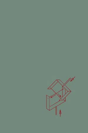 eBook - PDF
- Thomas R. Kane(Author)
- 2013(Publication Date)
- Academic Press(Publisher)
In this proposition, motions of the earth are left out of account. As knowledge of kinematics is prerequisite to understanding a 146 Static Equilibrium; SECTION 4.6 quantitative description of the errors thus introduced, further consideration of this question is deferred to Vol. II. Equations based on 3.6(a) or 3.6.1 are called force equations; those based on 3.6.5 or 3.6.6, moment equations. The term equilib-rium equation applies to all of them. Problem: A steel sphere (specific weight 489 lb/ft 3 ) is attached to an inclined board by means of a screw, as shown in Fig. 4.6a. FIG. 4.6a FIG. 4.6b Regarding the sphere and that portion of the screw which is outside of the board as a body B in contact over a surface σ (see Fig. 4.6b) with a body B' consisting of the remainder of the screw and a portion of the board, describe the system of contact forces exerted on B by B' across σ. Solution: The system of all gravitational forces exerted on B by other bodies in the universe is approximately equivalent to a single force (see 4.4.5) of magnitude 489 X iw(^y = 32 lb and having the line of action shown in Fig. 4.6c. (The mass center and the weight of B are taken to be those of the steel sphere, it being assumed that the screw's volume is so small, in comparison with the sphere's, that errors introduced by neglecting any possible difference in the mass densities of the screw and sphere are neg-ligible.) Static Equilibrium; SECTION 4.6 147 FIG. 4.6C The only body with which B is in contact is B'. In accordance with 3.5.6, the system of all contact forces exerted on B by B f across σ can be replaced with a couple of torque T and a single force F whose line of action passes through the point P shown in Fig.
Index pages curate the most relevant extracts from our library of academic textbooks. They’ve been created using an in-house natural language model (NLM), each adding context and meaning to key research topics.