A Primer for Spatial Econometrics

With Applications in R

G. Arbia

• Editore: Palgrave Macmillan
• Anno: 2014
• ISBN:
  9781137317940
• Argomento: Volkswirtschaftslehre
• Categoria: Ökonometrie

This book aims at meeting the growing demand in the field by introducing the basic spatial econometrics methodologies to a wide variety of researchers. It provides a practical guide that illustrates the potential of spatial econometric modelling, discusses problems and solutions and interprets empirical results.

1

The Classical Linear Regression Model

1.1 The basic linear regression model

Let us consider the following linear model

_n y₁ = _n X_kk β₁ + _n ε₁ (1.1)

where

is a vector of n observations of the dependent

variable y,

a matrix of n observations on k – 1

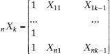
non-stochastic exogenous regressors including a constant term,

a vector of k unknown parameters to be estimated and

a

vector of stochastic disturbances. We will assume throughout the book that the n observations refer to territorial units such as regions or countries.

The classical linear regression model assumes normality, identicity and independence of the stochastic disturbances conditional upon the k regressors. In short

ε | X ≈ i.i.d.N (0, σ²_{ε n} I_n) (1.2)

_n I_n being an n-by-n identity matrix. Equation (1.2) can also be written as:

E(ε | X) = 0(1.3)

E(εε^T | X) = σ²_{ε n} I_n (1.4)

Equation (1.3) corresponds to the assumption of exogeneity, Equation (1.4) to the assumption of spherical disturbances (Greene, 2011).

Furthermore it is assumed that the k regressors are not perfectly dependent on one another (full rank of matrix X). Under this set of hypotheses the Ordinary Least Squares fitting criterion (OLS) leads to the best linear unbiased estimators (BLUE) of the vector of parameters β, say

_OLS =

. In fact the OLS criterion requires:

S(β) = e^T e = min (1.5)

where e = y – X

are the observed errors and e^T indicates the transpose of e.

From Equation (1.5) we have:

whence:

_OLS = (X^T X)^-1 X^T y (1.6)

As said the OLS estimator is unbiased

E(

_OLS | X) = β (1.7)

with a variance

Var(

_OLS | X) = (X^T X)^–1σ²_ε (1.8)

which achieves the minimum among all possible linear estimators (full efficiency) and tends to zero when n tends to infinity (weak consistency).

From the assumption of normality of the stochastic disturbances, normality of the estimators also follows:

_OLS | X ≈ N[β; (X^T X)^–1 σ²_ε] (1.9)

Furthermore, from the assumption of normality of the stochastic disturbances, it also follows that the alternative estimators, based on the Maximum Likelihood criterion (ML), coincide with the OLS solution.

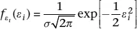
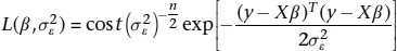
In fact, the single stochastic disturbance is distributed as:

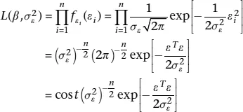
f being a density function, and consequently the likelihood of the observed sample is:

(1.10)

from the assumption of independence of the disturbances. From (1.1) we have that

ε = y – Xβ (1.11)

hence (1.10) can be written as:

(1.12)

and the log-likelihood as:

(1.13)

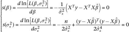
The scores functions are defined as:

(1.14)

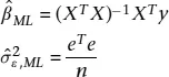
and solving the system of k + 1 equations, we have:

(1.15)

Thus, under the hypothesis of normality of residuals, the ML estimator of β coincides with the OLS estimator. The ML estimator of

on the contrary differs from the unbiased estimator

and it is biased, but asymptotically unbiased.

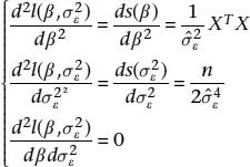
To ensure that the solution obtained is a maximum we consider the second derivatives:

(1.16)

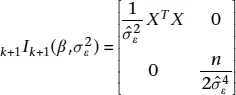
which can be arranged in the Fisher’s Information Matrix:

(1.17)

which is positive definite.

The equivalence between the ML and the OLS estimators ensures that the solution found enjoys all the large sample properties of the ML estimators, that is to say: asymptotic normality, consistency, asymptotic unbiasedness, full efficiency with respect to a larger class of estimators other than the linear...

Indice dei contenuti

• Cover
• Title
• Copyright
• Contents
• List of Figures
• List of Examples
• Foreword by William Greene
• Preface and Acknowledgements
• 1 The Classical Linear Regression Model
• 2 Some Important Spatial Definitions
• 3 Spatial Linear Regression Models
• 4 Further Topics in Spatial Econometrics
• 5 Alternative Model Specifications for Big Datasets
• 6 Conclusions: What’s Next?
• Solutions to the Exercises
• Index