Physics
Op Amp Gain
Op Amp Gain refers to the amplification factor of an operational amplifier (op amp). It represents the ratio of the output voltage to the input voltage. The gain of an op amp is a crucial parameter in determining the amplification capability and performance of the circuit in which it is used.
Written by Perlego with AI-assistance
Related key terms
1 of 5
10 Key excerpts on "Op Amp Gain"
 eBook - PDF
- Jiri Dostal(Author)
- 2013(Publication Date)
- Newnes(Publisher)
Parti The Operational Amplifier This page intentionally left blank 1. Basic Concepts 1.1 The Operational Amplifier The operational amplifier is a versatile amplifying device, originally intended for use in analog computers to perform linear mathematical operations. Forty years of development of the operational amplifier's internal circuit design reflects, to a significant extent, the development of electronic components from vacuum tubes to monolithic integrated circuits. An increasing refinement of the operational amplifier's properties has shifted the emphasis of its ap-plications from laboratories to industry. Due to its high performance, ver-satility, and low price, the operational amplifier now dominates the field of analog electronic systems. We generally define the operational amplifier as a direct-coupled amplifier with a high gain and a low level of inherent noise, capable of stable operation in a closed-feedback loop. The exact meaning of these characteristics will be given in Chapters 2 and 11. It should be mentioned here that the term direct-coupled does not imply an upper limitation of the amplifier's frequency re-sponse but, on the contrary, an extension of the operating range to zero frequency, or infinitely long periods. The direction of signal flow from input to output in an operational amplifier is given by the triangular shape of its symbol in Figure 1-la. Three of the four illustrated terminals represent the three signal terminals of an actual operational amplifier. These are the inverting input, noninverting input, and output. The fourth signal terminal, the ground, may be either actual (Figure 1—lb) or only virtual (power supply common in Figure 1-lc). In either case, it represents symbolically a group of at least two terminals intended for the supply of energy.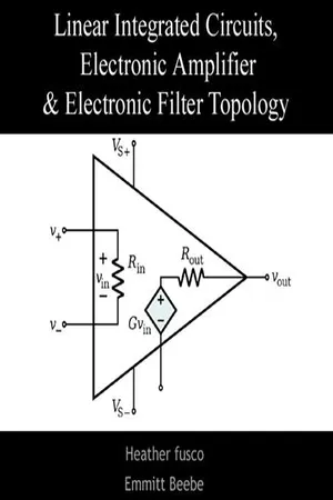 No longer available |Learn more
- (Author)
- 2014(Publication Date)
- College Publishing House(Publisher)
In the first approximation op-amps can be used as if they were ideal differential gain blocks; at a later stage limits can be placed on the acceptable range of parameters for each op-amp. Circuit design follows the same lines for all electronic circuits. A specification is drawn up governing what the circuit is required to do, with allowable limits. For example, the gain may be required to be 100 times, with a tolerance of 5% but drift of less than 1% in a specified temperature range; the input impedance not less than one megohm; etc. A basic circuit is designed, often with the help of circuit modeling (on a computer). Specific commercially available op-amps and other components are then chosen that meet the design criteria within the specified tolerances at acceptable cost. If not all criteria can be met, the specification may need to be modified. A prototype is then built and tested; changes to meet or improve the specification, alter functionality, or reduce the cost, may be made. ____________________ WORLD TECHNOLOGIES ____________________ Basic single stage amplifiers Non-inverting amplifier An op-amp connected in the non-inverting amplifier configuration In a non-inverting amplifier, the output voltage changes in the same direction as the input voltage. The gain equation for the op-amp is: However, in this circuit V – is a function of V out because of the negative feedback through the R 1 R 2 network. R 1 and R 2 form a voltage divider, and as V – is a high-impedance input, it does not load it appreciably. Consequently: where Substituting this into the gain equation, we obtain: Solving for V out : If A OL is very large, this simplifies to ____________________ WORLD TECHNOLOGIES ____________________ . Inverting amplifier An op-amp connected in the inverting amplifier configuration In an inverting amplifier, the output voltage changes in an opposite direction to the input voltage. No longer available |Learn more
- (Author)
- 2014(Publication Date)
- Academic Studio(Publisher)
In the first approximation op-amps can be used as if they were ideal differential gain blocks; at a later stage limits can be placed on the acceptable range of parameters for each op-amp. Circuit design follows the same lines for all electronic circuits. A specification is drawn up governing what the circuit is required to do, with allowable limits. For example, the gain may be required to be 100 times, with a tolerance of 5% but drift of less than 1% in a specified temperature range; the input impedance not less than one megohm; etc. A basic circuit is designed, often with the help of circuit modeling (on a computer). Specific commercially available op-amps and other components are then chosen that meet the design criteria within the specified tolerances at acceptable cost. If not all criteria can be met, the specification may need to be modified. A prototype is then built and tested; changes to meet or improve the specification, alter functionality, or reduce the cost, may be made. ____________________ WORLD TECHNOLOGIES ____________________ Basic single stage amplifiers Non-inverting amplifier An op-amp connected in the non-inverting amplifier configuration In a non-inverting amplifier, the output voltage changes in the same direction as the input voltage. The gain equation for the op-amp is: However, in this circuit V – is a function of V out because of the negative feedback through the R 1 R 2 network. R 1 and R 2 form a voltage divider, and as V – is a high-impedance input, it does not load it appreciably. Consequently: where Substituting this into the gain equation, we obtain: Solving for V out : If A OL is very large, this simplifies to . ____________________ WORLD TECHNOLOGIES ____________________ Inverting amplifier An op-amp connected in the inverting amplifier configuration In an inverting amplifier, the output voltage changes in an opposite direction to the input voltage. No longer available |Learn more
- (Author)
- 2014(Publication Date)
- University Publications(Publisher)
In the first approximation op-amps can be used as if they were ideal differential gain blocks; at a later stage limits can be placed on the acceptable range of parameters for each op-amp. Circuit design follows the same lines for all electronic circuits. A specification is drawn up governing what the circuit is required to do, with allowable limits. For example, the gain may be required to be 100 times, with a tolerance of 5% but drift of less than 1% in a specified temperature range; the input impedance not less than one megohm; etc. A basic circuit is designed, often with the help of circuit modeling (on a computer). Specific commercially available op-amps and other components are then chosen that meet the design criteria within the specified tolerances at acceptable cost. If not all criteria can be met, the specification may need to be modified. A prototype is then built and tested; changes to meet or improve the specification, alter functionality, or reduce the cost, may be m ade. ____________________ WORLD TECHNOLOGIES ____________________ Basic single stage amplifiers Non-inverting amplifier An op-amp connected in the non-inverting amplifier configuration In a non-inverting amplifier, the output voltage changes in the same direction as the input voltage. The gain equation for the op-amp is: However, in this circuit V – is a function of V out because of the negative feedback through the R 1 R 2 network. R 1 and R 2 form a voltage divider , and as V – is a high-impedance input, it does not load it appreciably. Consequently: where Substitu ting this into the gain equation, we obtain: Solving for V out : If A OL is very large, this simplifies to . ____________________ WORLD TECHNOLOGIES ____________________ Inverting amplifier An op-amp connected in the inverting amplifier configuration In an inverting amplifier, the output voltage changes in an opposite direction to the input voltage. eBook - PDF
- Behzad Razavi(Author)
- 2021(Publication Date)
- Wiley(Publisher)
What is the actual voltage gain? Let us now take into account the finite gain of the op amp. Based on the model shown in Fig. 8.1(b), we write (V in1 − V in2 )A 0 = V out , (8.10) 360 Chapter 8 Operational Amplifier as a Black Box and substitute for V in2 from Eq. (8.6): V out V in = A 0 1 + R 2 R 1 + R 2 A 0 . (8.11) As expected, this result reduces to Eq. (8.9) if A 0 R 2 ∕(R 1 + R 2 ) ≫ 1. To avoid confusion between the gain of the op amp, A 0 , and the gain of the overall amplifier, V out ∕V in , we call the former the “open-loop” gain and the latter the “closed-loop” gain. Equation (8.11) indicates that the finite gain of the op amp creates a small error in the value of V out ∕V in . If much greater than unity, the term A 0 R 2 ∕(R 1 + R 2 ) can be factored from the denominator to permit the approximation (1 + ) −1 ≈ 1 − for ≪ 1: V out V in ≈ ( 1 + R 1 R 2 ) [ 1 − ( 1 + R 1 R 2 ) 1 A 0 ] . (8.12) Called the “gain error,” the term (1 + R 1 ∕R 2 )∕A 0 must be minimized according to each application’s requirements. Example 8-3 A noninverting amplifier incorporates an op amp having a gain of 1000. Determine the gain error if the circuit is to provide a nominal gain of (a) 5, or (b) 50. Solution For a nominal gain of 5, we have 1 + R 1 ∕R 2 = 5, obtaining a gain error of: ( 1 + R 1 R 2 ) 1 A 0 = 0.5%. (8.13) On the other hand, if 1 + R 1 ∕R 2 = 50, then ( 1 + R 1 R 2 ) 1 A 0 = 5%. (8.14) In other words, a higher closed-loop gain inevitably suffers from less accuracy. Exercise Repeat the above example if the op amp has a gain of 500. With an ideal op amp, the noninverting amplifier exhibits an infinite input impedance and a zero output impedance. For a nonideal op amp, the I/O impedances are derived in Problem 8.6. 8.2.2 Inverting Amplifier Depicted in Fig. 8.7(a), the “inverting amplifier” incorporates an op amp along with resis- tors R 1 and R 2 while the noninverting input is grounded. No longer available |Learn more
- (Author)
- 2014(Publication Date)
- Academic Studio(Publisher)
In the first approximation op-amps can be used as if they were ideal differential gain blocks; at a later stage limits can be placed on the acceptable range of parameters for each op-amp. Circuit design follows the same lines for all electronic circuits. A specification is drawn up governing what the circuit is required to do, with allowable limits. For example, the gain may be required to be 100 times, with a tolerance of 5% but drift of less than 1% in a specified temperature range; the input impedance not less than one megohm; etc. A basic circuit is designed, often with the help of circuit modeling (on a computer). Specific commercially available op-amps and other components are then chosen that meet the design criteria within the specified tolerances at acceptable cost. If not all criteria can be met, the specification may need to be modified. A prototype is then built and tested; changes to meet or improve the specification, alter functionality, or reduce the cost, may be made. ____________________ WORLD TECHNOLOGIES ____________________ Basic single stage amplifiers Non-inverting amplifier An op-amp connected in the non-inverting amplifier configuration In a non-inverting amplifier, the output voltage changes in the same direction as the input voltage. The gain equation for the op-amp is: However, in this circuit V – is a function of V out because of the negative feedback through the R 1 R 2 network. R 1 and R 2 form a voltage divider , and as V – is a high-impedance input, it does not load it appreciably. Consequently: where Substi tuting this into the gain equation, we obtain: Solving for V out : If A OL is very large, this simplifies to . ____________________ WORLD TECHNOLOGIES ____________________ Inverting amplifier An op-amp connected in the inverting amplifier configuration In an inverting amplifier, the output voltage changes in an opposite direction to the input voltage. eBook - PDF
- G B Clayton(Author)
- 2013(Publication Date)
- Butterworth-Heinemann(Publisher)
Operational amplifiers have a very large open loop gain, which is determined by the product of the gains of the separate internal gain stages which go to make up the amplifier. If gain is expressed in dB the open loop frequency response plot for an amplifier is obtained as a result of linearly adding the Bode plots for the individual gain stages. Each stage follows a first order characteristic (see 2.4.1) and the final rate of attenuation and phase shift in the overall response is governed by the number of internal voltage gain stages. Two stages give a final roll off of 40 dB/decade and a phase shift approaching 180°; three stages give 60°/decade final roll off and a phase shift approaching 270°. In order that the open loop response of an operational amplifier shall exhibit a single 20 dB/decade roll off down to unity gain the frequency response of one of its internal stages must be made dominant. The break frequency associated with this dominant stage must be made sufficiently low to ensure that by its gain attenuation alone, it can get the loop gain magnitude down to unity at a frequency which is lower than that at which the other gain stages start to attenuate. In most present day integrated circuit designs very high individual stage gains are obtained by using active loads 1 and they are thus able to achieve a sufficiently large overall gain using only two internal voltage gain stages. Operational amplifiers of this type are normally frequency compensated by means of a single capacitor connected as a feedback capacitor around the second inverting voltage gain stage in the amplifier. The technique requires only small values of frequency compensating capacitor (10 pF-30 pF). Capacitors of this size are small enough to be fabricated on the same integrated circuit chip as the rest of the amplifier circuitry; this is the system normally adopted in most general purpose internally compensated amplifiers. No longer available |Learn more
- (Author)
- 2014(Publication Date)
- Research World(Publisher)
For example, an op-amp with a gain bandwidth product of 1 MHz would have a gain of 5 at 200 kHz, and a gain of 1 at 1 MHz. This low-pass characteristic is introduced deliberately, because it tends to stabilize the circuit by introducing a dominant pole. This is known as frequency compensation. Typical low cost, general purpose op-amps exhibit a gain bandwidth product of a few megahertz. Specialty and high speed op-amps can achieve gain bandwidth products of hundreds of megahertz. For very high-frequency circuits, a completely different form of op-amp called the current-feedback operational amplifier is often used. Other imperfections include: Finite bandwidth All amplifiers have a finite bandwidth. This creates several problems for op amps. First, associated with the bandwidth limitation is a phase difference between the ________________________ WORLD TECHNOLOGIES ________________________ input signal and the amplifier output that can lead to oscillation in some feedback circuits. The internal frequency compensation used in some op amps to increase the gain or phase margin intentionally reduces the bandwidth even further to maintain output stability when using a wide variety of feedback networks. Second, reduced bandwidth results in lower amounts of feedback at higher frequencies, producing higher distortion, noise, and output impedance and also reduced output phase linearity as the frequency increases. Input capacitance Most important for high frequency operation because it further reduces the open loop bandwidth of the amplifier. Non-linear imperfections Saturation output voltage is limited to a minimum and maximum value close to the power supply voltages. eBook - PDF
Fundamentals of Electronics
Book 1 Electronic Devices and Circuit Applications
- Thomas F. Schubert, Ernest M. Kim(Authors)
- 2022(Publication Date)
- Springer(Publisher)
1 C H A P T E R 1 Operational Amplifiers and Applications e Operational Amplifier (commonly referred to as the OpAmp) is one of the primary active devices used to design low and intermediate frequency analog electronic circuitry: its importance is surpassed only by the transistor. OpAmps have gained wide acceptance as electronic building blocks that are useful, predictable, and economical. Understanding OpAmp operation is funda- mental to the study of electronics. e name, operational amplifier, is derived from the ease with which this fundamental building block can be configured, with the addition of minimal external circuitry, to perform a wide variety of linear and non-linear circuit functions. Originally implemented with vacuum tubes and now as small, transistorized integrated circuits, OpAmps can be found in applications such as: signal processors (filters, limiters, synthesizers, etc.), communication circuits (oscillators, modulators, demodulators, phase-locked loops, etc.), Analog/Digital converters (both A to D and D to A), and circuitry performing a variety of mathematical operations (multipliers, dividers, adders, etc.). e study of OpAmps as circuit building blocks is an excellent starting point in the study of electronics. e art of electronics circuit and system design and analysis is founded on circuit realizations created by interfacing building block elements that have specific terminal character- istics. OpAmps, with near-ideal behavior and electrically good interconnection properties, are relatively simple to describe as circuit building blocks. Circuit building blocks, such as the OpAmp, are primarily described by their terminal char- acteristics. Often this level of modeling complexity is sufficient and appropriately uncomplicated for electronic circuit design and analysis. However, it is often necessary to increase the complexity of the model to simplify the analysis and design procedures. eBook - PDF
- Joseph J. Carr(Author)
- 2012(Publication Date)
- Academic Press(Publisher)
An example might be an instrumentation circuit that uses multiple out-puts, perhaps one to the A / D converter input of a digital computer and another to an analog oscilloscope or strip chart recorder. By buffering the analog output to the oscilloscope we prevent short circuits in the display wiring from affecting the signal to the computer, and vice versa. A special case of buffering is represented by using the unity-gain follower as a power driver. A long cable run may attenuate low-power signals. T o overcome this problem we sometimes use a low impedance power source to drive a long cable. This application points out the fact that a unity-gain follower actually does have power gain (the unity-gain feature refers only to the voltage gain). If the input impedance is typically much higher than the output impedance, yet V Q = V in , then by V 2 /R the delivered power output is much greater than the input power. Thus, the circuit of Fig. 12-26 is unity gain for voltage signals and greater-than-unity gain for power. It is therefore a power amplifier. T h e impedance transformation capability is obtained from the fact that an op-amp has a very high input impedance and a very low output impedance. Let us illustrate this application by a practical example. Figure 12-27A is a generic equivalent of a voltage source driving a load (R2). T h e resistance Rl represents the internal impedance of the signal source impedance. T h e signal voltage V is reduced at the output (y o ) by whatever voltage is dropped across source resistance Rl. T h e output voltage is found from V Q = V(R2)/(Rl + R2) ( 1 2 -4 7 ) By way of example: If the ratio of RI/R2 is, say, 10:1, then a 1-V D C potential is reduced to 0.091 V D C across R2. Ninety percent of the signal amplitude is lost. With a unity-gain noninverting amplifier, as in Fig.
Index pages curate the most relevant extracts from our library of academic textbooks. They’ve been created using an in-house natural language model (NLM), each adding context and meaning to key research topics.